Aitomistic Updates: Tools for analyzing your simulations

In this week’s newsletter, we’d like to highlight a powerful feature of MLatom (an open-source software supported by Aitomistic) as a tool for analysis of your calculations, e.g., with Gaussian. You can use prepare beautiful Jupyter notebooks and convert them into interactive the html files to browse together with your colleagues the molecules and spectra. You can use these materials instead of or in addition to your Supporting Information files in PDF. For this, **you can also use the Jupyter Lab on the **Aitomistic Hub.

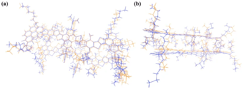
An example of this functionality is a web version of such a Jupyter Notebook for one of our publications: http://mlatom.com/misc/ita.html. In our study Alternating Donor–Acceptor Thienoacenes Featuring Up to 23 Linearly Fused Rings published in Org. Lett., earlier this year, we used the UAIQM extension of the AIQM2 method to optimize the 714-atom structure in ca. 88 min on 32 CPUs. Good luck doing that with DFT! The agreement with the crystallographic structure was quite good, given the flexibility of the noncovalently-bound complex with many alkyl groups. In this study, TD-DFT calculations were performed on smaller systems with Gaussian.

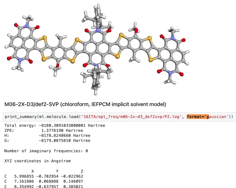
MLatom was then used to load the Gaussian output files and convert them to the molecule format as mol = ml.molecule.load(’myfile.log’, format=’gaussian’). Why is this important? It gives you a simple way to convert your old Gaussian calculations into a machine-readable database format with MLatom, which can be later used for training ML models. It is also easy to analyze calculations once loaded in Jupyter Notebook with MLatom, you can, e.g., view molecules by running a command in a cell mol.view().

You can use our Jupyter Notebook as http://mlatom.com/misc/ita.html as a template for your projects. It shows how to prepare summaries of calculations listing energies and thermochemical properties, number of imaginary frequencies, etc.

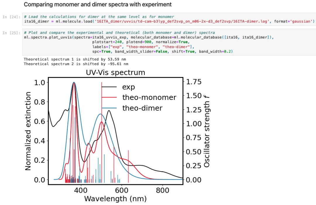
One particularly useful application is to analyze the UV/vis absorption spectra, which you can plot with MLatom’s built-in functions such as ml.spectra.plot_uvvis(molecule=mol, ...) (see tutorial) and compare to the experimental spectra, with functions for spectra alignment and plotting line spectra. Examples of how to print out the Tables for your SI with the list of excitations and their character are provided too.

Please also let us know what you would like us to improve to make your experiences with MLatom and Aitomistic better. Join us on Slack to directly chat with us.