MLatom 3.25: fine-tune the universal machine learning potentials on your own data

MLatom 3.25 is out with ultra-efficient fine-tuning of many of its zoo of universal machine learning potentials — AIQM, OMNI-P, ANI — on your own data. You train one of them on your own reference calculations, so that it reproduces the level of theory you actually work at while keeping the physics and the general behaviour it started with.

In 3.25 the whole family — the ANI models, AIQM1, AIQM2, AIQM3, UAIQM, OMNI-P1 and the excited-state OMNI-P2x — goes through the same train() call, and dispersion is declared once and handled on both sides. Here is what it is for, what it costs, and how to run it.

1. What it is for

A universal potential is built to work across chemistry in general. However, for your particular system at hand, it might be not good enough.

The usual options are both expensive: run everything at your reference level, or train a potential of your own from scratch. Fine-tuning is the third one. You give it a modest set of reference calculations on your system, and it adjusts the model you already trust to match them.

2. Six lines

One call, whichever potential you start from. Fine-tuning runs through the Python API:

import mlatom as ml

data  = ml.data.molecular_database.load('CH3NO2_100.json')
model = ml.models.methods(method='AIQM2')
model.train(molecular_database=data, property_to_learn='energy',
            dispersion_kwargs={'method': 'd4', 'functional': 'wb97x'},
            file_to_save_model='my_tl_model/')

model = ml.models.aiqm2.load('my_tl_model/')

You supply geometries with energies, and forces if you have them, at whatever level you trust.

A potential like AIQM2 is a sum of parts: a fast quantum-chemistry baseline, an explicit D4 dispersion term, and a neural network on top. Fine-tuning trains only the network, so MLatom subtracts the baseline and the dispersion from your reference energies first — the network learns just the difference — and adds them back when it predicts. That is what the dispersion_kwargs line declares.

Dispersion stays a formula rather than something the network learns, because a network only sees an atom's neighbours out to about 5 Å, and van der Waals attraction reaches further than that.

The result saves and loads like any other model, so you can put it straight into a geometry optimization, a transition-state search, frequencies and thermochemistry, or molecular dynamics.

3. What it costs

The worked example in the fine-tuning tutorial fine-tunes AIQM2 to reproduce B3LYP/6-31G* on ethanol. That target is a toy — chosen because it computes in seconds, not because it is more accurate than AIQM2. Example shows how closely fine-tuning reproduces your desired level.

As shipped, AIQM2 sits 1.37 kcal/mol away from that target on energies relative to the equilibrium structure. Thirty-five training geometries close it to 0.67, and at that size one fine-tuning takes ten to thirty seconds on a 2019 desktop — a GTX 1660 SUPER, a card with no tensor cores.

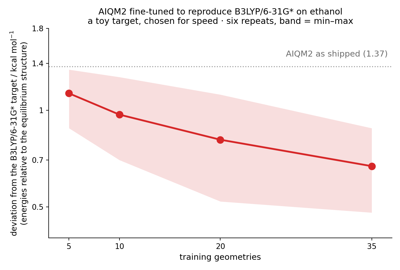Deviation from the target against training-set size. Every size is repeated six times and the band is the smallest to the largest of them, because at five geometries a single run is not a measurement — the scatter there is as wide as the step between sizes.

Ethanol is one small molecule; something larger or more flexible will want more than thirty-five geometries. What holds generally is the reason the requirement is modest at all: the AIQM2 network is a correction on top of a physical baseline, and fine-tuning freezes most of it and adjusts only the last layers. You are learning a small correction, not a potential — which is also why it runs on hardware this ordinary. Without a GPU the same fit is roughly two orders of magnitude slower; using the fine-tuned potential needs no GPU at all, and fifteen predictions came back in a second.

So if a universal potential is close but not quite right for your system, the fix is a handful of reference calculations and a coffee break.

4. Where each model lives

The ANI family, AIQM1, AIQM2, OMNI-P1 and OMNI-P2x are in open-source MLatom, and their weights download on first use. AIQM3 ships as a compiled add-on, aitomic-addons on PyPI, free for academic and non-commercial use with commercial use licensed separately. UAIQM currently runs on the Aitomistic Hub. All of them fine-tune through the same train() call, with the arguments each model needs.

python3 -m pip install --upgrade mlatom

That tutorial ships with a Jupyter notebook and the data set, so it runs as it stands.

Rather not install anything? MLatom also runs in your browser on the Aitomistic Hub, driven by Protomia — an AI assistant that carries out a whole simulation from a plain-language request. There is a free trial for everyone, including commercial use.

5. What else is in MLatom

Methods — universal ML potentials (ANI, AIMNet2) and AI-enhanced QM methods (UAIQM, AIQM1, AIQM2, AIQM3); DFT, semi-empirical and wavefunction methods through interfaces to PySCF, Gaussian, ORCA, xtb, MNDO, Turbomole, DFTB+, Sparrow and Columbus.
ML models — train your own ML potentials (KREG, GAP-SOAP, ANI, MACE and more) with active learning, Δ-learning, transfer learning, self-correction, and fine-tuning of the universal potentials.
Simulations — geometry optimization, transition-state search, IRC, frequencies and thermochemistry, molecular and nonadiabatic dynamics, IR/Raman/UV–vis spectra, and periodic boundary conditions.

Citation

When using fine-tuning, please cite:

Seyedeh Fatemeh Alavi, Yuxinxin Chen, Yi-Fan Hou, Fuchun Ge, Peikun Zheng, Pavlo O. Dral. ANI-1ccx-gelu Universal Interatomic Potential and Its Fine-Tuning: Toward Accurate and Efficient Anharmonic Vibrational Frequencies. J. Phys. Chem. Lett. 2025, 16, 483–493. DOI: 10.1021/acs.jpclett.4c03031