
Fine-tuning universal models
Note
New in MLatom 3.25.0. Upgrade with pip install --upgrade mlatom if you are
on an earlier version.
MLatom’s universal models — the ANI family, AIQM1, AIQM2, AIQM3, UAIQM, OMNI-P1 and the excited-state OMNI-P2x — are built to work across chemistry in general. For one particular system they are usually good, but there are always cases when it is desirable to improve the quality. If you have reference data of your own — geometries with energies, and optionally forces, at whatever level you trust — you can fine-tune a universal model on it. It keeps the model’s physics and general behaviour but reproduces your reference level.
This page covers fine-tuning the universal models. For transfer learning in general, including fine-tuning a model you trained yourself, see Transfer learning.
The whole thing, in six lines
Files for this example
finetuning.ipynb ·
CH3NO2_100.json — 100 nitromethane
geometries with reference energies and forces ·
both as a zip, so it runs as it
stands. The notebook is also shown with its output
at the bottom of this page.
import mlatom as ml

data = ml.data.molecular_database.load('CH3NO2_100.json')
model = ml.models.methods(method='AIQM2')
model.train(molecular_database=data, property_to_learn='energy',
            dispersion_kwargs={'method': 'd4', 'functional': 'wb97x'},
            file_to_save_model='my_tl_model/')

model = ml.models.aiqm2.load('my_tl_model/')   # and use it
That is a complete fine-tuning run. The rest of this page is what the arguments
mean, why dispersion_kwargs is there, and how to check the result — read it
when you need it.
The workflow is the same for every model: load your data, call train(), then
load the result and predict with it. What differs between models is what is
inside them, which is worth understanding before you start.
How these models are built
A universal model is a sum of parts. In the most general case:
\(E_\text{NN}\) is the neural network. In a model with a baseline it learns only the difference between the baseline and the target level, which is why these are called delta-learning models. With no baseline it has to describe the whole energy itself.
\(E_\text{dispersion}\) is an explicit D3 or D4 correction. A neural network only sees an atom’s neighbours out to a fixed cutoff — 5.1 Å for ANI-2x, 5.2 Å for the others — so long-range attraction is supplied by this formula rather than learned.
\(E_\text{baseline}\) is a fast quantum-chemistry method — GFN2-xTB* in AIQM2 and AIQM3, ODM2* in AIQM1. It supplies most of the physics.
Not every model has all three. Plain ANI is \(E_\text{NN}\) alone; OMNI-P1 is a network plus dispersion with no baseline; AIQM2 has all three.
Fine-tuning trains only \(E_\text{NN}\). The baseline and the dispersion term are calculated by the QM software, hence MLatom during training subtracts those terms from the reference data automatically to generate the delta database for training the NN:
You can provide this database yourself instead of waiting for MLatom to generate it (which is typically fast as baselines are cheap, but nonetheless).
The models
model |
composition |
delta-learning? |
needs installed |
|---|---|---|---|
|
NN |
no |
— |
|
NN + D4 |
no |
|
|
ODM2* + NN ensemble + D4 |
yes |
MNDO or Sparrow, |
|
ODM2* + NN ensemble |
yes |
MNDO or Sparrow |
|
GFN2-xTB* + Δ-NN ensemble + D4 |
yes |
|
|
GFN2-xTB* + Δ-NN ensemble |
yes |
|
|
GFN2-xTB* + Δ-NN ensemble + D3 |
yes |
|
|
GFN2-xTB* + Δ-NN ensemble |
yes |
|
UAIQM |
baseline + Δ-NN, or NN alone, per entry |
per entry |
per entry |
OMNI-P1 |
single NN + D4 |
no |
|
OMNI-P2x |
excited-state NN ensemble + oscillator-strength model |
no |
— |
The required model is simply set with method='AIQM2' and, for some models,
extra model-specific settings — as is done throughout MLatom for the
universal models.
OMNI-P2x is fine-tuned too, but through a call of its own: it is an excited-state model, so its data carries electronic states rather than one energy per geometry, and it has a second model for oscillator strengths. See OMNI-P2x below.
A complete example
The example below is the core of the notebook, which runs it on nitromethane from
start to finish: the fine-tuning itself, what it wrote, using the fine-tuned model,
reusing the delta database, and the dimer curves at the end of this page.
It needs the xtb and dftd4 programs
installed, since AIQM2 is built from a GFN2-xTB* baseline and a D4 dispersion term
and fine-tuning has to evaluate both over your geometries; MLatom finds them
through the xtbbin and dftd4bin environment variables. A D3 term needs the
s-dftd3 program and dftd3bin.
import mlatom as ml

db = ml.data.molecular_database.load('CH3NO2_100.json', format='json')

model = ml.models.methods(method='AIQM2')
    # model_index=0    # fine-tune one member of the ensemble instead of all eight -
                       # about eight times faster, but you lose the spread between
                       # members that gives you an uncertainty estimate.
                       # A list works too: [0, 1, 4]

model.train(
    molecular_database=db,
    property_to_learn='energy',
    xyz_derivative_property_to_learn='energy_gradients',  # omit this line to fit energies only
    dispersion_kwargs={'method': 'd4', 'functional': 'wb97x'},  # see "Dispersion" below
    file_to_save_model='my_tl_model/',
    # hyperparameters={'max_epochs': 200},   # how long to train. How much you need
                        # depends on your data; check that the loss has stopped
                        # improving rather than trusting any particular number
)
Note that model_index is given when you set the model up, not to train() —
it selects which of the eight pretrained networks you are starting from.
That one call leaves you a directory you can use straight away:
my_tl_model/
  cv0.pt … cv7.pt     the fine-tuned neural networks, one per ensemble member
  tree.json           what the model is made of, and how to rebuild it
  delta_db.h5         the training data, with everything that went into it
and prints what it built:
Fine-tuned model composition: E = GFN2-xTB* + dNN + D4(wb97x)
Using the fine-tuned model, now or in a later script:
model = ml.models.aiqm2.load('my_tl_model/')

mol = ml.data.molecule.from_xyz_file('nitromethane.xyz')
model.predict(molecule=mol, calculate_energy=True, calculate_energy_gradients=True)
print(mol.energy)
What is in the training database
delta_db.h5 is one file holding your reference energies, every term that was
subtracted from them, and the delta labels the networks were actually fitted to.
Each term is kept under its own name, so you can look at any of them:
db = ml.data.molecular_database.load('my_tl_model/delta_db.h5')

db[0].energy                              # your reference energy
db[0].get_property('gfn2xtbstar.energy')  # the baseline over that geometry
db[0].get_property('dispersion.energy')   # the dispersion term
db[0].delta_energy                        # what the network was fitted to

db.label_sources                          # what each of those names means
Which names are present follows from what the model is made of, not from its
name: a baseline only for AIQM1, AIQM2, AIQM3 and the UAIQM entries that have
one; a dispersion term only where one was declared. db.label_sources always
tells you.
Keeping the parts and not only their difference buys three things:
You can check the arithmetic yourself — \(\Delta E = E - E_\text{dispersion} - E_\text{baseline}\), molecule by molecule.
Trying a different dispersion choice on the same geometries costs nothing, because the baseline — the expensive part of preparing the data — is already there. See Reusing the delta database.
You do not pay for the baseline twice if you change a training setting and run again.
If any of those calculations fails, MLatom says so rather than carrying on: a geometry whose baseline or dispersion energy came back missing or as NaN is reported, with a count and the indices, instead of silently becoming a NaN in the delta database and being trained on.
Building the delta database can also be parallelized trivially, because the QM
calculations for the individual molecules are independent and can be run at the
same time on an HPC cluster. That is why you can build it yourself and hand it
over rather than waiting for train() to do it.
What your data needs
A molecular_database whose molecules carry geometries and a reference energy;
add forces if you want the model to reproduce those too. Energies are in Hartree
and gradients in Hartree/Å, as elsewhere in MLatom. Your data must contain only
elements the model supports — H, C, N, O for AIQM1, OMNI-P1, and the ANI-1x
family, more for others.
Dispersion
If the model you are fine-tuning has no dispersion term — plain ANI-1x,
ANI-1ccx, ANI-2x, ANI-1xnr, or any @DFT* variant — none of this applies.
Leave dispersion_kwargs out and skip to the next section.
For the models that do have one there is a real decision to make, and MLatom asks you to make it rather than choosing on your behalf. Fine-tuning has to settle what the network is being asked to reproduce: your reference energies as they stand, or your reference energies with the dispersion term subtracted. And if dispersion is subtracted from them, the fine-tuned model has to add the same term back when it predicts — otherwise it returns something other than the level you trained it on.
dispersion_kwargs settles both halves at once: the term you name is
subtracted from your reference energies and added back when the model
predicts. Because it is the same term in both places, your reference energies
are reproduced whichever term you choose. What the choice actually decides is how
much of the model is a physical formula rather than a neural network, and
therefore how the model behaves away from the geometries you trained on.
You give it one of these:
what you write |
what it means |
|---|---|
|
D4 with the ωB97X parameters: subtracted from your reference data, and present in the fine-tuned model |
|
no dispersion anywhere — nothing subtracted, and the fine-tuned model has no dispersion term |
|
as above, but with damping parameters you supply instead of the functional’s own |
You must always say which method. {'functional': 'b3lyp'} on its own does not
say whether D3 or D4 is meant, nor which D3 damping form, so what came out of your
reference data could differ from what goes back into the model. The choices are
d4, and the D3 forms d3bj, d3zero, d3bjm, d3zerom, d3op.
A functional name is not always the same numbers
The dispersion term is computed by dftd4 or s-dftd3, programs you install
separately, and a functional name in those programs can come to mean different
parameters in a later version. It has happened: up to dftd4 3.7.0 the name
wb97x selected the parameters fitted for ωB97X (Chai and Head-Gordon, 2008);
from dftd4 4.0.0 the same name selects ωB97X-D4 (Najibi and Goerigk, 2020), a
different functional. On one nitromethane the two differ by 3.5 kcal/mol, and
they roughly double the well depth of a methane dimer.
MLatom pins the parameters for wb97x, so that name means the same thing here on
every dftd4 version, and the models built against it — AIQM1, AIQM2, OMNI-P1, the
-D4 ANI variants — are unaffected. For any other functional you name, you get
whatever your installed program has. Two consequences worth knowing:
Your own results stay self-consistent. The same term is subtracted from your reference data and added back when the model predicts, so your reference energies are reproduced whatever your program computes.
A delta database and a fine-tuned model belong to the program that made them. Prepare labels on one machine and predict on another with a different dispersion program, and the term added back is not the term that was subtracted. The provenance stamp records the program version for this reason —
db.label_sources['delta']shows it — so you can tell, but nothing checks it for you.
If that matters for your work, give the numbers rather than the name:
{'method': 'd3bj', 'functional': 'b3lyp', 'damping_function_params': [...]}
fixes the term exactly, on any version.
There is no default: train() stops with an error if you leave
dispersion_kwargs out for a model that has a dispersion term. Any default would
quietly do the wrong thing for somebody — assuming the model’s own term would add
D4 for someone fine-tuning on plain ωB97X, and assuming none would strip the
long-range physics for someone fine-tuning on MP2.
What the choice costs you is shown on a fine-tuned model further down, in How does it behave far from your data?.
Choosing the term for your reference level
Your level has no dispersion (plain B3LYP, plain ωB97X). Both of these are self-consistent, and they give you different models:
dispersion_kwargs=False                                    # reproduces your level exactly, with no
                                                           # long-range attraction - as your level behaves

dispersion_kwargs={'method': 'd4', 'functional': 'b3lyp'}  # see the warning below -
                                                           # usually NOT what you want here
Declaring a dispersion term does not add dispersion to your level. The same term is subtracted from your reference data and added back at prediction, so on your data the model reproduces B3LYP either way. It is not a route from B3LYP data to a B3LYP-D4 model — for that you need B3LYP-D4 reference data.
What the second line does change is the behaviour away from your data. The NN
cancels the D4 term wherever it can, which is inside its cutoff and within the
range of geometries you trained on; beyond that it cannot, so an uncancelled D4
tail survives. The result is B3LYP at short range with a D4 tail at long range —
neither B3LYP nor B3LYP-D4. For a reference level that genuinely has no
dispersion, use False.
Your level’s dispersion can be separated (B3LYP-D3(BJ) and similar). Name the same correction your reference calculation used:
dispersion_kwargs={'method': 'd3bj', 'functional': 'b3lyp'}
Your level’s dispersion cannot be separated (MP2, CCSD(T) — there dispersion is not an additive term at all). Use the model’s own:
dispersion_kwargs={'method': 'd4', 'functional': 'wb97x'}    # AIQM1, AIQM2, OMNI-P1, ANI-*-D4
dispersion_kwargs={'method': 'd3bj', 'functional': 'b973c'}  # AIQM3
This is more than a convention. D4(ωB97X) is the correction the pretrained network was fitted against in the first place, so keeping it means the layers that are held fixed still describe what they were trained to describe. Use each model’s own term — D3(BJ)/B97-3c for AIQM3, not D4(ωB97X).
Be clear about what you then have: a model that reproduces MP2 where you trained it and has D4(ωB97X) behaviour at long range. It is not MP2 far from your training geometries, and is worth describing that way in a paper.
ωB97X-D and similar. ωB97X-D uses a D2 correction, which MLatom does not
compute — only D3 and D4 are available. The cleanest route is to fine-tune to
plain ωB97X, the functional without its dispersion correction, and use
{'method': 'd4', 'functional': 'wb97x'}. That is the parameterisation the
pretrained network assumes, and D4 describes long range better than D2 did. If
your reference data is fixed and must stay ωB97X-D, treat the level as inseparable
and use the model’s own term. As with B3LYP above, that does not turn your data
into something else: the model still reproduces ωB97X-D where you trained it. What
changes is out-of-domain, where D4 rather than the original D2 supplies the
long-range attraction.
Loading a fine-tuned model
Every family has its own loader, taking the directory train() wrote:
model = ml.models.aiqm2.load('my_tl_model/')          # or aiqm1, aiqm3, uaiqm, omnip1
model = ml.models.ani_methods.load('my_tl_model/')    # the ANI family
model = ml.models.load('my_tl_model/tree.json')       # or the generic loader
Per-model settings
Only the second column differs from the worked example; everything else is the same call.
model |
set it up with |
worth knowing |
|---|---|---|
ANI |
|
no baseline, so only dispersion (if any) is subtracted |
AIQM1 |
|
Sparrow also works |
AIQM2 |
|
as in the worked example |
AIQM3 |
|
its own dispersion term is D3(BJ)/B97-3c, not D4 |
UAIQM |
|
entries are baseline + Δ-NN or NN alone; the model works out which |
OMNI-P1 |
|
one NN, no ensemble, so |
OMNI-P2x |
|
excited-state model — different data and a different call, see below |
Shared defaults, for every model above: the first and third layers of each NN are
held fixed (fixed_layers=[[0, 4]]), and the per-element atomic-energy shift is
refitted from your reference data — your level’s atomic references are not the
model’s, and that difference is a constant per composition which the NN should not
have to absorb. max_epochs defaults to 100, which is a starting value and not a
recommendation: how long you need depends on how much data you have and how far
your reference level sits from the model’s, so watch the loss rather than trust a
number. Override any of these through hyperparameters.
OMNI-P2x
OMNI-P2x is an excited-state model, and three things about it differ from everything above.
Your data carries electronic states, not one energy. Each molecule holds
mol.electronic_states, with an energy per state, and mol.oscillator_strengths
if you want to fine-tune those too. nstates says how many states to train on.
There is no baseline and no dispersion term, so dispersion_kwargs does not
apply — the network describes the excited-state energies itself.
There are two models, and they are named separately rather than written into one directory: an ensemble of three energy models, and one oscillator-strength model that is only trained if you ask for it.
model = ml.models.methods(method='OMNI-P2x')

model.train(
    molecular_database=db,      # molecules carrying electronic_states
    nstates=2,                  # how many electronic states to train on
    train_osc=True,             # also fine-tune the oscillator-strength model
    en_model_filename='OMNI-P2x_ft_emodel',
    osc_model_filename='OMNI-P2x_ft_osc_model',
    xyz_derivative_property_to_learn='energy_gradients',   # optional
    hyperparameters={'max_epochs': 100},
)
Its own defaults are max_epochs=100, fixed_layers=[[0, 4]] as elsewhere, and
gap_coefficient=0.01 — how much weight the gaps between states carry relative to
the state energies themselves. Fine-tuning the oscillator-strength model sets
gap_coefficient to zero, since oscillator strengths have no gaps to preserve.
Two worked examples, with data and notebooks, are on the OMNI-P2x page: fine-tuning for the nuclear-ensemble approximation, and active transfer learning for non-adiabatic dynamics.
Other training settings
hyperparameters accepts more than max_epochs:
setting |
what it does |
|---|---|
|
molecules per gradient step |
|
step size; see the note below |
|
training stops once the rate has decayed this far |
|
how long to wait without improvement before reducing the rate, and by how much |
|
how much weight forces carry relative to energies |
|
how the losses are combined and monitored |
|
which layers are held fixed |
|
OMNI-P2x only: how much weight the gaps between electronic states carry relative to the state energies |
The full set is in the API documentation.
Their defaults are those of the underlying trainer, which was written for training a network from scratch. Fine-tuning generally wants gentler settings — a smaller learning rate above all, since you are adjusting a model that has already converged rather than fitting one from nothing. We do not recommend particular values here: doing that honestly would take a study across models and data sizes, and that has not been done. Treat the defaults as a starting point and watch the loss.
Reusing the delta database
Rather than always computing the delta database inside train(), you can build it
once — however and wherever suits you — and then hand it over. These routines live
in ml.delta_learning: delta learning is a general idea, not something specific to
the AIQM family, and the module knows about baselines and dispersion terms rather
than about which model happens to use them.
delta_db = ml.delta_learning.prepare_delta_database(
    db, method='AIQM2',
    dispersion_kwargs={'method': 'd4', 'functional': 'wb97x'},
    xyz_derivative_property_to_learn='energy_gradients')
delta_db.dump('prepared_labels.h5')

model = ml.models.methods(method='AIQM2')
model.train(delta_db='prepared_labels.h5', file_to_save_model='my_tl_model/')
delta_db= takes either a filename or a database. Note that the second call says
nothing about dispersion: every delta database records what was subtracted from it
— the baseline, the dispersion term, the program that computed it, and whether
forces were handled too — and train() reads that instead of asking you to repeat
yourself. If you do pass dispersion_kwargs as well it must name the same term, or
train() stops with an error. A database carrying no such record is refused rather
than guessed at.
To try a different dispersion choice on the same data without recomputing the
baseline, point baseline_db= at the database you already have — the baseline is
kept in it under its own name:
delta_b = ml.delta_learning.prepare_delta_database(
    db, method='AIQM2',
    dispersion_kwargs={'method': 'd3bj', 'functional': 'b3lyp'},
    baseline_db='my_tl_model/delta_db.h5')
How much data do you need?
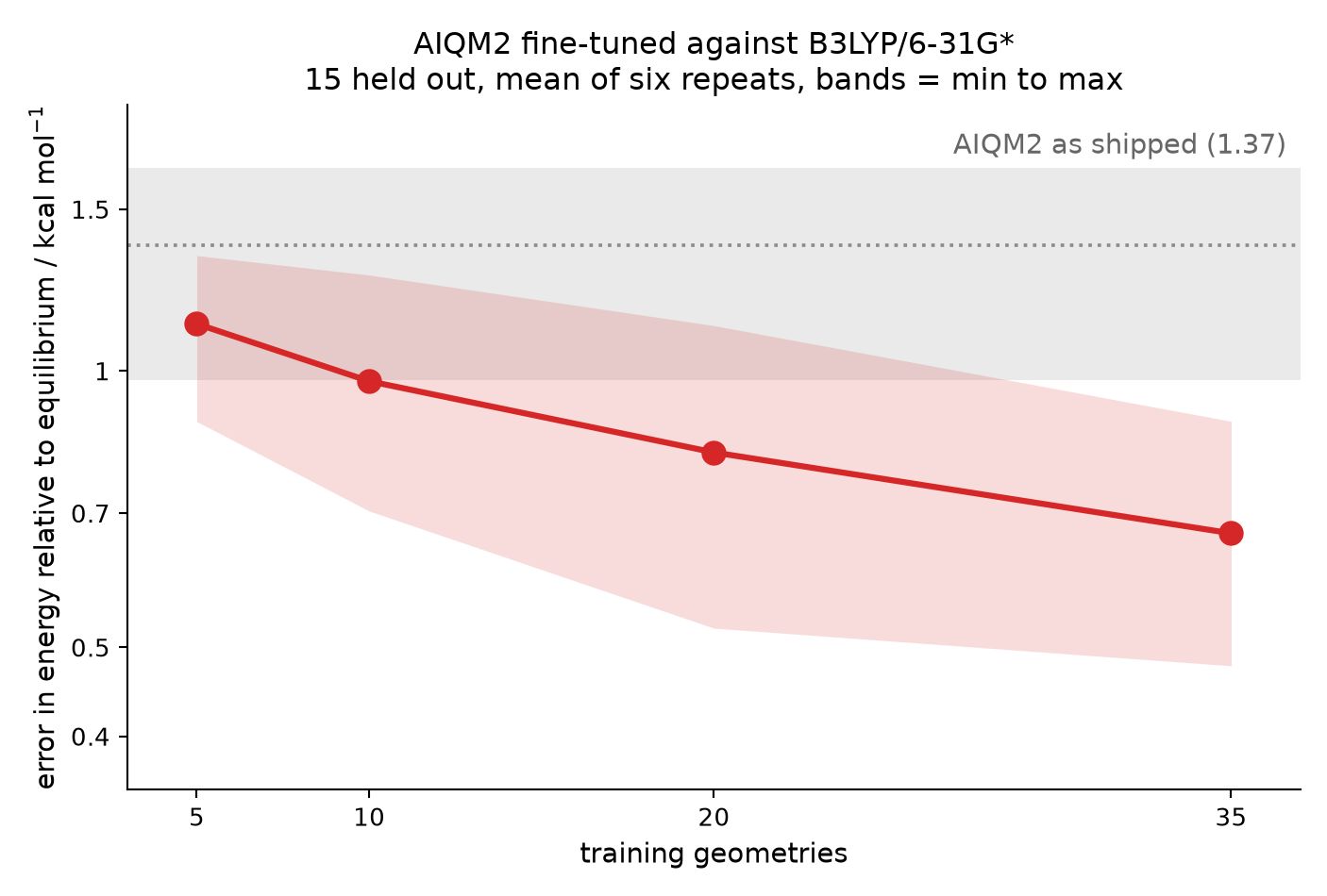
Enough to be worth the reference calculations, and that is usually less than people expect. The runs below are AIQM2 (one ensemble member) fine-tuned against B3LYP/6-31G* energies, computed with PySCF, for 50 Wigner-sampled ethanol geometries spanning 38 kcal/mol. Fifteen are held out and never trained on, and the whole experiment is repeated six times, each time with a different draw of which geometries are held out and which are trained on.
Files for this section
finetuning_ethanol.ipynb —
already run, so you can read its output without running anything ·
ethanol_50.json — the 50 geometries with
B3LYP/6-31G* energies ·
ethanol_eq.json — the optimized structure
the errors are measured from ·
all three as a zip
Everything here comes out of that notebook, seed and all, so you can re-run it rather than take these numbers on trust.
training geometries |
error / kcal mol⁻¹ |
|---|---|
AIQM2 as shipped |
1.37 (0.98–1.66) |
5 |
1.13 (0.88–1.34) |
10 |
0.97 (0.70–1.27) |
20 |
0.81 (0.52–1.12) |
35 |
0.67 (0.48–0.88) |
Each entry is the mean over the six repeats, with the smallest and the largest of them in brackets.
What is being measured. Energies are taken relative to the optimized equilibrium structure — the same fixed geometry for every model — so what is compared is the cost of distorting away from equilibrium, which is the quantity you would actually use. Taking a difference this way also removes the arbitrary offset between two methods’ absolute energies: AIQM2 and B3LYP/6-31G* do not put the zero of energy in the same place, and for a single molecule that difference is simply a constant, of no interest to anyone.
That reference structure is the ethanol_eq.json above. It is not one of the sampled geometries —
Wigner sampling displaces every one of them, and the closest still sits about
10 kcal/mol above the minimum — so it has to be the optimized structure rather
than the lowest sample.
What the numbers say. The gain is real but gradual: 1.37 kcal/mol as shipped, 1.13 at five geometries, and 0.67 by thirty-five. Five is within the run-to-run spread of the shipped model and should not be read as an improvement on its own. Each step after that helps, and none of them is dramatic — this is a fit getting steadily better, not a threshold being crossed.
Why six repeats and not one. A single fine-tuning run at these sizes is not a measurement. Even the shipped model — the same model every time — spans 0.98 to 1.66 kcal/mol across the repeats, because the fifteen geometries it is graded on change. The fine-tuned runs move for that reason and because they saw different training geometries as well. At every size the spread is comparable to the step between one size and the next, so one run at one size can come out flat, or backwards, on the draw alone.
Your own numbers will differ with the system, the reference level and how much of the surface your geometries cover, which is why the next section is about measuring them rather than trusting these.
Checking your fine-tuned model
Does it reproduce the data you trained it on? Predict on your training molecules and compare. The difference should be at the level of the fit, i.e. rather small compared to typical errors of QM simulations.
import numpy as np

check = db.copy(atomic_labels=['xyz_coordinates'], molecular_labels=[])
model.predict(molecular_database=check, calculate_energy=True)
error = np.abs(np.array(check.get_properties('energy'))
               - np.array(db.get_properties('energy')))
print(f'max |E_predicted - E_reference| = {error.max():.6f} Hartree')
molecular_labels=[] matters here: without it the copy carries your reference
energies across, and a molecule the model failed on would keep the reference value
and appear to have zero error.
How does it behave far from your data? Plot a dimer dissociation curve out to about 12 Å, against your reference and against the model you started from. A model with no dispersion term goes flat beyond its cutoff, 5.1–5.2 Å, where the network stops seeing its neighbours. An averaged error over a training set of small molecules will never show you this, and it is exactly the regime most applications depend on.
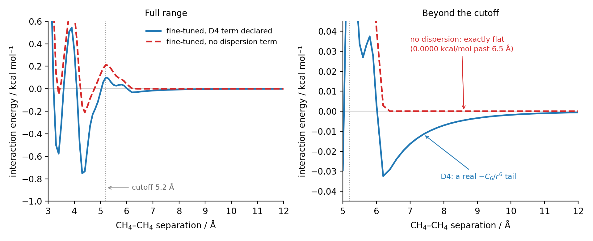
Both curves are the same model fine-tuned on the same data, differing only
in whether dispersion_kwargs named a term. Past the cutoff the difference is
absolute: the model with no dispersion term is exactly flat — 0.0000 kcal/mol
beyond 6.5 Å, while the one with D4 keeps a real \(-C_6/r^6\) tail
(−0.024 kcal/mol at 6.6 Å, −0.006 at 8.2 Å, −0.0008 at 11.4 Å). Nothing in a
training set of small molecules will tell you which of those you have.
The notebook runs this
same comparison on its own nitromethane data — it fine-tunes the model twice, with and
without a declared dispersion term, and plots both panels — so you can reproduce
it rather than take these curves on trust.
The oscillations below 5 Å are worth seeing too, and they are not the dispersion term’s doing: this model was fine-tuned on ethanol geometries and is being asked about two separated methanes, which is outside anything it was shown. That is the same warning as the paragraph above, made visible.
Two rigid methane molecules pulled apart, computed with the plain ANI-1x
ensemble. There is a proper minimum at 3.45 Å (−0.73 kcal/mol), but beyond 6 Å the
interaction energy is 0.01 kcal/mol and falling to zero — the network sees nothing
past its cutoff, so there is no long-range attraction at all. This is what a
dispersion term supplies, and what its absence costs. Run the same curve with your
own reference level on the same axes: that comparison is the diagnostic, and this
single curve only shows the tail it is meant to expose.
The whole example, run
The notebook from the top of this page, with its output — the fine-tuning run, what it wrote, the fine-tuned model in use, and the dispersion comparison it ends on.
Fine-tuning universal models
This notebook is the worked example from the Fine-tuning universal models tutorial, with the data set bundled so it can be run as it stands.
We fine-tune AIQM2 on 100 nitromethane geometries with reference energies and forces, look at what training wrote, and check the result.
What you need installed: MLatom, and the xtb and dftd4 programs — AIQM2 is
built from a GFN2-xTB* baseline, a neural-network correction and a D4 dispersion
term, and fine-tuning has to evaluate the first and the third over your geometries.
import os
import numpy as np
import mlatom as ml

print('MLatom', ml.__version__)
The reference data
CH3NO2_100.json holds 100 nitromethane geometries, each with an energy and
forces. Your own data needs the same: a molecular_database whose molecules carry
geometries and a reference energy, plus forces if you want the model to reproduce
those too. Energies are in Hartree and gradients in Hartree/Å.
db = ml.data.molecular_database.load('CH3NO2_100.json', format='json')

print(f'{len(db)} molecules, {len(db[0].atoms)} atoms each')
print('elements:', sorted(set(db[0].element_symbols)))

energies = np.array(db.get_properties('energy'))
print(f'energies: {energies.min():.4f} .. {energies.max():.4f} Hartree')
print('gradients on the first molecule:',
      np.shape(db[0].get_xyz_vectorial_properties('energy_gradients')))
Fine-tuning
One call. Two things are worth pointing at:
dispersion_kwargsnames the dispersion term. It is subtracted from your reference energies and added back when the model predicts — the same term in both places, so your reference energies are reproduced whichever you choose. There is no default, because any default would quietly do the wrong thing for somebody. AIQM2's own term is D4 with the ωB97X parameters.model_indexis given when you set the model up, not totrain(). It selects which of the eight pretrained networks you start from; leaving it out fine-tunes all eight, which is about eight times slower but gives you the spread between members as an uncertainty estimate.
max_epochs is set low here so the notebook runs quickly. It is not a
recommendation — how long you need depends on your data, so watch the loss rather
than trust a number.
model = ml.models.methods(method='AIQM2', model_index=0)

model.train(
    molecular_database=db,
    property_to_learn='energy',
    xyz_derivative_property_to_learn='energy_gradients',   # omit to fit energies only
    dispersion_kwargs={'method': 'd4', 'functional': 'wb97x'},
    file_to_save_model='my_tl_model/',
    hyperparameters={'max_epochs': 20},
)
The last line printed is what the fine-tuned model is made of. It should read
Fine-tuned model composition: E = GFN2-xTB* + dNN + D4(wb97x)
which is the same decomposition as the equation at the top of the tutorial: a baseline, a neural network, and a dispersion term.
print(sorted(os.listdir('my_tl_model')))
What training wrote
delta_db.h5 is one file holding your reference energies, every term that was
subtracted from them, and the delta labels the network was actually fitted to.
Each term is kept under its own name.
prepared = ml.data.molecular_database.load('my_tl_model/delta_db.h5')

print('label sources in this database:')
for name, spec in sorted(prepared.label_sources.items()):
    print(f'  {name:14s} {spec}')
mol = prepared[0]

reference  = float(mol.energy)
baseline   = float(mol.get_property('gfn2xtbstar.energy'))
dispersion = float(mol.get_property('dispersion.energy'))
delta      = float(mol.delta_energy)

print(f'reference   E          = {reference:14.6f} Hartree')
print(f'baseline    GFN2-xTB*  = {baseline:14.6f}')
print(f'dispersion  D4(wb97x)  = {dispersion:14.6f}')
print(f'delta       what the NN learns = {delta:14.6f}')
print()
print('E - baseline - dispersion == delta:',
      np.isclose(reference - baseline - dispersion, delta))
That last line is the point of keeping the parts and not only their difference: $\Delta E = E - E_\text{dispersion} - E_\text{baseline}$ is checkable, molecule by molecule. It also means the baseline — the expensive part of preparing the data — is already computed if you want to try something else on the same geometries.
Using the fine-tuned model
tuned = ml.models.aiqm2.load('my_tl_model/')

check = db.copy(atomic_labels=['xyz_coordinates'], molecular_labels=[])
tuned.predict(molecular_database=check, calculate_energy=True)

error = np.abs(np.array(check.get_properties('energy'))
               - np.array(db.get_properties('energy')))
print(f'max  |E_predicted - E_reference| = {error.max():.6f} Hartree')
print(f'mean |E_predicted - E_reference| = {error.mean():.6f} Hartree')
molecular_labels=[] matters here. Without it the copy carries your reference
energies across, and a molecule the model failed on would keep the reference value
and appear to have zero error.
For comparison, the model before fine-tuning:
stock = ml.models.methods(method='AIQM2', model_index=0)

before = db.copy(atomic_labels=['xyz_coordinates'], molecular_labels=[])
stock.predict(molecular_database=before, calculate_energy=True)

error_before = np.abs(np.array(before.get_properties('energy'))
                      - np.array(db.get_properties('energy')))
print(f'stock AIQM2      mean |dE| = {error_before.mean():.6f} Hartree'
      f'  ({error_before.mean() * 627.5094740631:8.3f} kcal/mol)')
print(f'fine-tuned       mean |dE| = {error.mean():.6f} Hartree'
      f'  ({error.mean() * 627.5094740631:8.3f} kcal/mol)')
Plotted, with the constant offset taken out of both so the shape is what you see. The page shows the same comparison on a set with a wider energy range; this one is your training data, so it is the easy case.
%matplotlib inline
import matplotlib.pyplot as plt

K = 627.5094740631
reference = np.array(db.get_properties('energy'))
tuned_e   = np.array(check.get_properties('energy'))
stock_e   = np.array(before.get_properties('energy'))

# energies relative to each set's own mean: the constant offset between your
# reference level and the model is not the interesting part, the shape is
rel = lambda e: (e - e.mean()) * K

fig, ax = plt.subplots(figsize=(4.6, 4.4))
lo = min(rel(reference).min(), rel(tuned_e).min()) - 0.02
hi = max(rel(reference).max(), rel(tuned_e).max()) + 0.02
ax.plot([lo, hi], [lo, hi], color='0.75', lw=0.9, zorder=0)
ax.scatter(rel(reference), rel(stock_e), s=26, marker='s', alpha=0.75,
           color='#d62728', label='AIQM2 as shipped')
ax.scatter(rel(reference), rel(tuned_e), s=26, alpha=0.85,
           color='#1f77b4', label='fine-tuned')
ax.set_xlabel('reference energy / kcal mol$^{-1}$')
ax.set_ylabel('predicted / kcal mol$^{-1}$')
ax.set_xlim(lo, hi); ax.set_ylim(lo, hi)
ax.legend(frameon=False, fontsize=9, loc='upper left')
ax.set_title('energies relative to each set mean', fontsize=10)
fig.tight_layout()
plt.show()

Most of the difference is a constant offset: your reference level's atomic energies are not AIQM2's. Fine-tuning refits that per-element shift from your data, which is why it should not be left for the network to absorb.
Reusing the prepared data
Rather than recomputing the baseline every time, hand the prepared database over.
train() reads what was subtracted from it — the baseline, the dispersion term,
the program that computed it, and whether forces were handled too — instead of
asking you to say it again.
delta_db = ml.delta_learning.prepare_delta_database(
    db, method='AIQM2',
    dispersion_kwargs={'method': 'd4', 'functional': 'wb97x'},
    xyz_derivative_property_to_learn='energy_gradients')

delta_db.dump('prepared_labels.h5', format='h5')

again = ml.models.methods(method='AIQM2', model_index=0)
again.train(delta_db='prepared_labels.h5',
            file_to_save_model='reuse_model/',
            hyperparameters={'max_epochs': 5})
To try a different dispersion choice on the same geometries, point baseline_db=
at the database you already have. Watch the output: it computes the new dispersion
term and not the baseline.
delta_b = ml.delta_learning.prepare_delta_database(
    db, method='AIQM2',
    dispersion_kwargs={'method': 'd3bj', 'functional': 'b3lyp'},
    baseline_db='my_tl_model/delta_db.h5')

a = np.array(delta_db.get_properties('delta_energy'))
b = np.array(delta_b.get_properties('delta_energy'))
print(f'delta with D4(wb97x)     = {a[0]:.6f} Hartree')
print(f'delta with D3(BJ)/b3lyp  = {b[0]:.6f} Hartree')
Behaviour far from your data
The check above says the model reproduces what you trained it on. It says nothing about what happens elsewhere, and that is where a dispersion term earns its place.
A neural network sees an atom's neighbours only out to a fixed cutoff — 5.2 Å for most of these models. Beyond that it contributes nothing, so a fine-tuned model with no dispersion term has no long-range attraction at all.
Here is that difference, measured the only way that settles it: the same model
fine-tuned on the same data twice, differing only in whether dispersion_kwargs
named a term.
CH4 = np.array([[ 0.0000,  0.0000,  0.0000],
                [ 0.6276,  0.6276,  0.6276],
                [ 0.6276, -0.6276, -0.6276],
                [-0.6276,  0.6276, -0.6276],
                [-0.6276, -0.6276,  0.6276]])
Z = np.array([6, 1, 1, 1, 1])

separations = np.concatenate([np.arange(3.0, 6.01, 0.1),
                              np.arange(6.2, 12.01, 0.2)])

def dimer_curve(model):
    dimers = ml.data.molecular_database()
    for r in separations:
        dimers.molecules.append(ml.data.molecule.from_numpy(
            coordinates=np.vstack([CH4, CH4 + np.array([r, 0, 0])]),
            species=np.concatenate([Z, Z])))
    monomer = ml.data.molecular_database(
        [ml.data.molecule.from_numpy(coordinates=CH4, species=Z)])
    model.predict(molecular_database=dimers, calculate_energy=True)
    model.predict(molecular_database=monomer, calculate_energy=True)
    return (np.array(dimers.get_properties('energy'))
            - 2 * monomer[0].energy) * K
curves = {}
for label, dispersion in (('fine-tuned, D4 term declared',
                           {'method': 'd4', 'functional': 'wb97x'}),
                          ('fine-tuned, no dispersion term', False)):
    m = ml.models.methods(method='ANI-1x', model_index=0)
    m.train(molecular_database=db, property_to_learn='energy',
            dispersion_kwargs=dispersion,
            file_to_save_model=f'ft_{bool(dispersion)}',
            hyperparameters={'max_epochs': 100}, verbose=0)
    curves[label] = dimer_curve(m)
    beyond = np.abs(curves[label][separations >= 6.5]).max()
    print(f'{label:32s} largest |E| beyond 6.5 A: {beyond:.4f} kcal/mol')
fig, (full, tail) = plt.subplots(1, 2, figsize=(9.6, 3.9))
for ax in (full, tail):
    ax.axhline(0, color='0.8', lw=0.8, zorder=0)
    ax.axvline(5.2, color='0.55', lw=1.0, ls=':', zorder=0)

for (label, values), style, colour in zip(curves.items(), ('-', '--'),
                                          ('#1f77b4', '#d62728')):
    full.plot(separations, values, style, lw=1.9, color=colour, label=label)
    keep = separations >= 5.0
    tail.plot(separations[keep], values[keep], style, lw=1.9, color=colour)

full.set_xlim(3, 12); full.set_ylim(-1.0, 0.6)
full.set_title('Full range', fontsize=10)
full.legend(frameon=False, fontsize=8.5, loc='upper right')
tail.set_xlim(5, 12); tail.set_ylim(-0.045, 0.045)
tail.set_title('Beyond the cutoff', fontsize=10)
for ax in (full, tail):
    ax.set_xlabel('CH$_4$–CH$_4$ separation / Å')
    ax.set_ylabel('interaction energy / kcal mol$^{-1}$')
fig.tight_layout()
plt.show()

Past the cutoff the difference is absolute. The model with no dispersion term is exactly flat — the printout above gives 0.0000 kcal/mol beyond 6.5 Å — while the one with D4 keeps a real $-C_6/r^6$ tail. Nothing in a training set of small molecules would have told you which of those you had.
The oscillations below 5 Å are worth seeing too, and they are not the dispersion term's doing: this model was fine-tuned on nitromethane and is being asked about two separated methanes, which is outside anything it was shown. That is the same warning as the paragraph above, made visible.
When using this feature, please cite
Seyedeh Fatemeh Alavi, Yuxinxin Chen, Yi-Fan Hou, Fuchun Ge, Peikun Zheng, Pavlo O. Dral. ANI-1ccx-gelu Universal Interatomic Potential and Its Fine-Tuning: Toward Accurate and Efficient Anharmonic Vibrational Frequencies. J. Phys. Chem. Lett. 2025, 16, 483–493. DOI: 10.1021/acs.jpclett.4c03031. Preprint on ChemRxiv: https://doi.org/10.26434/chemrxiv-2024-c8s16 (2024-10-09).