
Data
Here we show how to use MLatom to deal with data. There are three major data types in MLatom: molecules, databases of molecules, and MD trajectories, which are shown below (figure from MLatom 3 paper under CC-BY license):
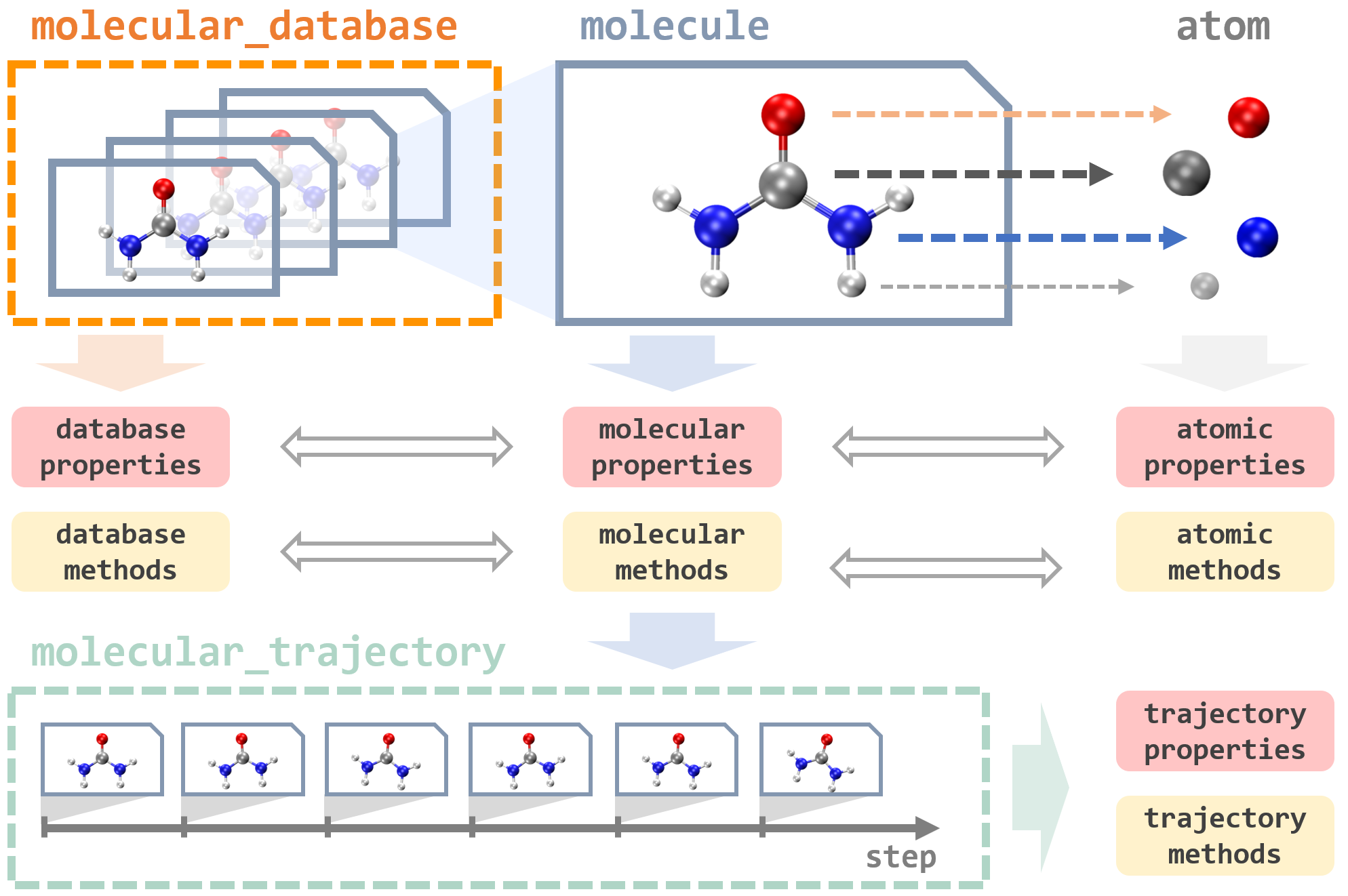
If you are looking for data rather than for the data structures, see our overview of what is available and how to choose:
Arif Ullah, Yuxinxin Chen, Pavlo O. Dral. Molecular quantum chemical data sets and databases for machine learning potentials. Mach. Learn.: Sci. Technol. 2024, 5, 041001. DOI: 10.1088/2632-2153/ad8f13.
Data sets released by our group that are often used with MLatom:
Lina Zhang, Shuang Zhang, Alec Owens, Sergei N. Yurchenko, Pavlo O. Dral. VIB5 database with accurate ab initio quantum chemical molecular potential energy surfaces. Sci. Data 2022, 9, 84. DOI: 10.1038/s41597-022-01185-w.
Max Pinheiro Jr, Shuang Zhang, Pavlo O. Dral, Mario Barbatti. WS22 database: combining Wigner Sampling and geometry interpolation towards configurationally diverse molecular datasets. Sci. Data 2023, 10, 95. DOI: 10.1038/s41597-023-01998-3.
Before running examples below in Python/Jupyter notebook, you need to add and run the line import mlatom as ml as usual. We also provide a short video introduction about data objects used in MLatom:
Molecules
Molecule is a central concept in MLatom as most of operations are usually done on molecule class objects. This objects store the information about the constituents atom objects, their coordinates, and any property we want to learn or calculate. Molecules can be loaded and dumped in various formats.
Creating and loading molecule
A molecule object can be created from scratch. A very explicit way (not used in practice!) relecting how the molecule is actually constructed is the following:
mol = ml.molecule()
atom1 = ml.data.atom(atomic_number=1, xyz_coordinates=[0.0, 0.0, 0.0])
mol.atoms.append(atom1)
...
In practice, you can create the molecule using many useful functions. E.g., you can load it from SMILES string and the geometry will be generated and optimized with Pybel’s make3D() method:
mol = ml.molecule()
mol.read_from_smiles_string('CCCCCCC')
print(mol.xyz_coordinates)
...
In above example, you can see how to access the XYZ coordinates stored in a molecule object.
Very common way is to load the geometry from XYZ coordinates. There are several ways to do it. You can either provide XYZ coordinates as a string, read them from file or from numpy array:
mol = ml.molecule()
mol.read_from_xyz_string('''2

H 0 0 0
H 0 0 0.74
''')
# or
mol.read_from_xyz_file('h2.xyz')
# or
import numpy as np
xyz = np.array([[0, 0, 0], [0, 0, 0.7]])
mol.read_from_numpy(coordinates=xyz, species=np.array([1, 1]))
...
A small nuance is that if you remove read_ from above methods, you can directly get the molecule object, i.e., compare:
mol = ml.molecule()
mol.read_from_xyz_file('h2.xyz')
# or
mol = ml.molecule.from_xyz_file('h2.xyz')

# also works:
mol = ml.molecule.from_smiles_string('CCCCCCC')
mol = ml.molecule.from_numpy(coordinates=xyz, species=np.array([1, 1]))
Also, you can read XYZ files in different formats. The default one is:
first line: number of atoms
second line: blank or comments
following lines: element symbol or atomic number followed by x, y, z coordinates in Angstrom
MLatom also supports reading XYZ files in Columbus, Newton-X, and Turbomole formats, just add format, e.g., as mol = ml.molecule.from_xyz_file('h2.xyz', format='Newton-X').
Dumping and loading
Ultimately, molecule is a data format. Hence, it is convenient to dump and load it as such, e.g., in json format:
mol.dump(filename='h2.json')
mol2.load(filename='h2.json')
print(mol, mol2)
You can also save the coordinates in text file:
mol.write_file_with_xyz_coordinates('h2.xyz')
or load the molecule from Gaussian output file and dump it later:
mol = ml.molecule.load('gaussian_output_file.log', format='gaussian')
mol.dump('parsed_molecule.json', format='json')
Properties
You can access, modify, and add different properties.
Some of the most common examples are charge and multiplicity:
mol.charge = 1
mol.multiplicity = 2
We have already saw how to access xyz coordinates. In the same way, we can access other properties (if they are availble, of course…), e.g.:
# examples of accessing properties
xyz = mol.xyz_coordinates
print(mol.energy)
print(mol.energy_gradients)
mol.hessian
# modifying properties
mol.energy = 3.00
mol.energy_gradients = np.array(...)
A bit more complicated are properties corresponding to different electronic states (see a dedicated tutorial on excited-state data format). They are stored in molecule.electronic_states which is a list of molecule objects themselves, corresponding to each state (note that by default this list is empty – it is only filled either after the excited-state calculations or by the user). This allows to access a property of any state the same way as accessing a property of a ‘normal’ molecule object. For example:
# let's get S1 state
S1 = mol.electronic_states[1]
print(f'Energy of S1 state is {S1.energy}')
print(f'Its forces are')
print(-S1.energy_gradients)
print(f'checking multiplicity: {S1.multiplicity}')
Where a label came from
The same geometry often has labels from more than one source – a DFT energy and a coupled-cluster energy, or a raw energy and a delta correction. A molecule can say which one its labels are at:
mol.label_source = 'wb97x'
This is a plain name and it can be anything you find useful: a method, a basis,
a delta, 'experiment'. MLatom does not interpret it; it records it, keeps it
through dumping and loading, and lets you ask for a property by its source:
mol.energy                                  # the label in use
mol.get_property('wb97x.energy')            # from a named source
mol.get_property('ccsd_t.energy_gradients') # any property, any source
A dotted name that does not exist raises rather than returning NaN, so a
misspelled source is reported instead of quietly becoming a missing value.
For that to work, each source’s labels have to be kept under its own name and not
only in mol.energy:
# an energy at another level: filed under 'ccsd_t' and put in use
mol.set_label_source('ccsd_t', energy=-1.17123)

# a level with gradients as well
wb97x = ml.data.properties_tree_node(name='wb97x')
wb97x.energy = -1.16453
wb97x.energy_gradients = np.array([[0.0, 0.0, 0.02871], [0.0, 0.0, -0.02871]])
mol.wb97x = wb97x
Which sources a molecule carries:
mol.label_sources_present()
This is what lets one geometry be trained at several levels of theory at once – see fine-tuning for models that take the level as an input. A complete example of a database built this way is below.
Other useful methods
Above overview is just to explain the key features when dealing with molcules. There is much more to it, which you can check out in the manual:
getting xyz string for printing it
calculating and rescaling kinetic energy
getting internuclear distances (for a pair and all pairs of atoms)
copying molecules with or without indicated properties
getting smiles (
molecule.smiles)rotating, translating, scaling, and aligning
printing detailed info (with
molecule.info())getting numpy array with electronic state energies, gradients, energy gaps, and excitation energies
dealing with generic vectorial properties (e.g., dipole moments)
and some others more technical methods.
Molecular databases
We often have to deal with a collection of molecular objects, which are stored in the
molecular_database class instances. The molecules are stored in the list molecular_database.molecules.
Molecular databases are in many respects extension of the molecule class, e.g., they can be loaded and dumped in a similar manner:
# prepare H2 geometries with bond lengths ranging from 0.5 to 5.0 Å
xyz = np.zeros((451, 2, 3))
xyz[:, 1, 2] = np.arange(0.5, 5.01, 0.01)
z = np.ones((451, 2)).astype(int)
molDB = ml.molecular_database.from_numpy(coordinates=xyz, species=z)

molDB.dump(filename='h2.json')
molDB2 = ml.molecular_database.load(filename='h2.json')
The useful feature of molecular databases is that they can be manipulated as lists/numpy arrays:
print(len(molDB))           # 451
print(len(molDB[:100:4]))   # 25
A related feature is that a database can be split into several other databases (useful, e.g., for splitting into training and test sets):
# let's change the splitting to 9:1 instead of default 8:2
train, test = molDB.split(fraction_of_points_in_splits=[0.9, 0.1])
Molecular databases also provide an easy acccess to the properties of all molecules, e.g., if we want to get the list of some property and save them in a text file, we can use:
molDB.get_properties(property_name='energy')
molDB.write_file_with_properties('h2.energies', property_name='energy')
There are also options to dump gradients and other vectorial properties as well as other useful technical features, see the manual.
Databases can also be written in HDF5, which is worth using once they get large – it is much smaller and faster to read back than json:
molDB.dump(filename='h2.h5', format='h5')
molDB2 = ml.molecular_database.load(filename='h2.h5')
dump() still defaults to json, so nothing changes unless you ask for h5.
load() works out the format from the file name, so it needs no format.
Label sources in a database
A database records which sources its labels come from, so a file carries its own provenance instead of relying on a file name or on someone’s memory:
molDB.set_label_source('wb97x')       # every molecule in the database
molDB.label_sources                   # what it holds, and what is known about each

# describe a source in as much or as little detail as you have
molDB.register_label_source('ccsd_t', program='MRCC', basis='cc-pVTZ')
The registry survives dumping, loading and splitting: a training and a validation set split off the same database both keep it, so a split set still knows what it is. Databases from different sources can be combined and the registry merges.
Dropping molecules that lack a label
A molecule with no value for the property being learned would enter the loss as
NaN and quietly damage training. To keep only the ones that can be learned
from:
usable = molDB.without_missing_labels('energy')
MLatom’s own training paths call this for you, on the validation set as well as the training set. It is here because it is also useful directly, e.g. after parsing a batch of outputs where some jobs failed.
Building a database with two levels of theory, by hand
Everything above, in one example: three H2 geometries, each labelled at two levels of theory, saved to a file and read back. The numbers stand in for your own calculations – nothing here computes them, the database only stores them.
import numpy as np
import mlatom as ml

# bond length in Angstrom, wB97X energy and its derivative, CCSD(T) energy
rows = [(0.70, -1.16453, -0.02871, -1.17123),
        (0.74, -1.16612,  0.00034, -1.17284),
        (0.80, -1.16389,  0.02043,  None)]     # this one has no CCSD(T) yet

molDB = ml.molecular_database()
for r, e_dft, dedr, e_cc in rows:
    mol = ml.molecule.from_numpy(coordinates=np.array([[0.0, 0.0, 0.0],
                                                       [0.0, 0.0, r]]),
                                 species=np.array([1, 1]))

    # the wB97X energy and gradients, under their own name
    wb97x = ml.data.properties_tree_node(name='wb97x')
    wb97x.energy = e_dft
    wb97x.energy_gradients = np.array([[0.0, 0.0, -dedr], [0.0, 0.0, dedr]])
    mol.wb97x = wb97x

    # the CCSD(T) energy, under its own name; no gradients at this level
    if e_cc is not None:
        ccsd_t = ml.data.properties_tree_node(name='ccsd_t')
        ccsd_t.energy = e_cc
        mol.ccsd_t = ccsd_t

    # the labels in use are the wB97X ones
    mol.energy = e_dft
    mol.energy_gradients = wb97x.energy_gradients
    mol.label_source = 'wb97x'

    molDB.molecules.append(mol)

# what those names mean, said once for the whole database
molDB.register_label_source('wb97x', method='wB97X', basis='6-31G*', program='PySCF')
molDB.register_label_source('ccsd_t', method='CCSD(T)', basis='cc-pVTZ', program='MRCC')

molDB.dump(filename='h2_two_levels.h5', format='h5')
Read back, the labels are where you left them and the file itself says what they are:
db = ml.molecular_database.load(filename='h2_two_levels.h5')

db.label_sources
# {'wb97x': {'method': 'wB97X', 'basis': '6-31G*', 'program': 'PySCF'},
#  'ccsd_t': {'method': 'CCSD(T)', 'basis': 'cc-pVTZ', 'program': 'MRCC'}}

db[0].label_source                            # 'wb97x' -- the labels in use
db[0].energy                                  # -1.16453
db[0].get_property('wb97x.energy')            # -1.16453, the same number by name
db[0].get_property('ccsd_t.energy')           # -1.17123
db[0].get_property('wb97x.energy_gradients')  # [[0, 0, 0.02871], [0, 0, -0.02871]]
db[0].label_sources_present()                 # ['ccsd_t', 'wb97x']

db.get_properties('ccsd_t.energy')            # [-1.17123 -1.17284 nan]
The third geometry has no coupled-cluster energy, so a model trained at that level has to leave it out:
trainable = db.without_missing_labels('ccsd_t.energy')
#   1 of 3 molecules dropped: no usable ccsd_t.energy
A label that was never computed reads back as NaN from an h5 file and as an
absent source from a json one; without_missing_labels treats the two alike.
MD trajectories
MD trajectories are a common data type and are handled with the molecular_trajectory class in MLatom. They consist of molecular_trajectory_step objects which contain information about molecule and other information such as step number, time, energies, etc.:
traj = ml.data.molecular_trajectory()
...
print(f'Info for MD trajectory step {traj.steps[5].step}'')
print(f'Molecule: {traj.steps[5].molecule}')
print(f'Time: {traj.steps[5].time}')
print(f'Kinetic energy: {traj.steps[5].molecule.kinetic_energy}')
The trajectories can be dumped and loaded as different formats: json (easier to open and browse, but heavy and slow, dumping overwrites the file), h5md (faster, smaller, dumping appends, not overwrites), plain text (xyz coordinates, velocities, energies, temperature, etc., dumping overwrites):
traj.dump(filename='mytraj.h5md', format='h5md')
traj2.load(filename='mytraj.h5md', format='h5md')
To unlock many of the features available in molecular databases, it is often convenient to convert the trajectory into molecular_database:
moldb = traj.to_database()
Visualizing data objects
You can use the common tools for visualizing XYZ files, etc. Additionally, MLatom provides several handy routines for quick checks of data objects in Jupyter notebooks:
my_molecule.view()
my_molecular_database.view()
my_trajectory.view()
and also for vibrations, see below.
Visualizing vibrations
There are several ways to visualize the vibrations:
At the end of the calculations via input file/command line using the options
freq,ir, orraman, MLatom will dump thefreq_gaussian{mol_index}.logfile, which uses Gaussian-style output format for frequencies. You can open it in ChemCraft.You can also dump text output file using Gaussian-style format for frequencies from the Python API:
mymolecule.dump(filename='gauss.log', format='gaussian').You can directly view the vibrations in
Jupyter notebookby usingmymolecule.view(normal_mode=...), as shown below for an examplemolvibr.jsonfile:
import mlatom as ml
# let's load the molecule with the required properties
molvibr = ml.molecule()
molvibr.load(filename='molvibr.json')
# choose the normal mode to visualize
normal_mode = 1
# let's view it
molvibr.view(normal_mode=normal_mode)
You appear to be running in JupyterLab (or JavaScript failed to load for some other reason). You need to install the 3dmol extension:
jupyter labextension install jupyterlab_3dmol
# we can also check the information for this normal mode
print(f'Frequency:   {molvibr.frequencies[normal_mode]:.2f} cm^-1')
print(f'Normal mode in Angstrom')
for atom in molvibr.atoms:
    disp = atom.normal_modes[normal_mode]
    print(f" {disp[0]:8.3f} {disp[1]:8.3f} {disp[2]:8.3f}")
Frequency:   288.70 cm^-1
Normal mode in Angstrom
   -0.000    0.000   -0.025
   -0.085    0.168   -0.141
    0.085   -0.168   -0.141
    0.000    0.000    0.184
   -0.000   -0.000   -0.003
    0.018   -0.021   -0.014
   -0.018    0.021   -0.014
    0.000    0.000    0.085
   -0.000   -0.000   -0.890
# the non-displaced geometry for reference
print(molvibr.get_xyz_string())
9

C            -1.2121068000000          -0.2252488500000           0.0000164100000
H            -1.2701429600000          -0.8599818400000          -0.8855315500000
H            -1.2701264500000          -0.8599834500000           0.8855643400000
H            -2.0710636400000           0.4504289000000           0.0000252100000
C             0.0804149500000           0.5556635800000           0.0000041500000
H             0.1395635900000           1.1970970800000          -0.8856250600000
H             0.1395848700000           1.1970854800000           0.8856411200000
O             1.1428329300000          -0.3971737900000          -0.0000106600000
H             1.9796722200000           0.0702558200000          -0.0001121300000
# non-displaced geometry
molvibr.view()
You appear to be running in JupyterLab (or JavaScript failed to load for some other reason). You need to install the 3dmol extension:
jupyter labextension install jupyterlab_3dmol