OMNI-P2x
OMNI-P2x is the first universal excited-state potential, see details in the paper:
Mikołaj Martyka, Xin-Yu Tong, Joanna Jankowska, Pavlo O. Dral. OMNI-P2x: A Universal Neural Network Potential for Excited-State Simulations. 2025. Preprint on ChemRxiv: https://doi.org/10.26434/chemrxiv-2025-j207x (2025.04.16).
Model weights and additional scripts are available at https://github.com/dralgroup/omni-p2x.
Tutorials below are prepared by Mikołaj Martyka with modifications by Pavlo O. Dral.
Contents:
UV/vis spectra simulations with OMNI-P2x
Single-point convolution
Files for download:
Predicting UV-Vis Spectra with OMNI-P2x
This tutorial demonstrates how to use the OMNI-P2x universal neural network potential, available through MLatom, to predict UV-Vis absorption spectra of organic molecules. OMNI-P2x is trained to approximate TD-DFT/B3LYP-level excited-state properties — including excitation energies and oscillator strengths — at a fraction of the computational cost.
What you will learn
- How to load a molecular structure and optimize its geometry with AIQM3.
- How to predict excited-state properties (excitation energies & oscillator strengths) using OMNI-P2x.
- How to generate and plot a broadened UV-Vis spectrum.
- How to compare the ML-predicted spectrum against a reference TD-DFT calculation.
- The effect of the level of geometry optimizations on the spectra precision.
System: trans-azobenzene
We use ***trans-azobenzene** (C₁₂H₁₀N₂, 24 atoms) as our example molecule. Azobenzene is a classic photoswitchable chromophore with a symmetry-forbidden n→π\ transition in the visible region and a strong π→π* transition in the UV.
1. Setup
First, we import MLatom. If you are running this on your own machine, make sure MLatom is installed, with version ≥ 3.22.
import mlatom as ml
2. Load the molecular structure
We load the initial geometry of trans-azobenzene from a SMILES string. This is the starting point before geometry optimization.
mol = ml.data.molecule.from_smiles_string('C1=CC=C(C=C1)N=NC2=CC=CC=C2')
# of course, if you have file with xyz coordinates, you can load it to as
# mol = ml.data.molecule.from_xyz_file('azb.xyz')
mol.view()
3Dmol.js failed to load for some reason. Please check your browser console for error messages.
3. Geometry optimization with AIQM3
Before computing excited-state properties, we need to optimize the ground-state geometry. Importantly, OMNI-P2x is not recommended for geometry optimizations as it was not a focus of its parametrization. Using it to optimize geometries, or simulate spectra for molecules far-from-equlibrium will not be a good idea.
Since OMNI-P2x was trained on TD-DFT data on DFT (B3LYP/6-31+G*)-optimized geometries, OMNI-P2x is expected to perform best for geometries optimized at the same level of theory. However, geometry optimizations with DFT will take longer than OMNI-P2x excited-state calculations. Hence, if you want quick results, you might want to use one of many ML-based methods, sacrificing a bit of precisions for the lower cost. You will see later the influence of the geometry on the spectra, which is quite common also for the electronic-structure methods, not just OMNI-P2x.
In this tutorial, we will optimize the ground-state geometry using AIQM3 — a general-purpose neural network potential for ground-state energies and forces approaching coupled-cluster accuracy. You can try many of the other universal potentials MLatom provides. AIQM3 itself is available via add-ons to MLatom and can also be run on online platforms (Aitomistic Hub at https://aitomistic.xyz and Aitomistic Lab@XMU at https://atom.xmu.edu.cn), while many other methods (AIQM2, etc.) are available after properly installing MLatom with the required dependences.
Here we will also use the geomeTRIC optimizer, as it is free and open-source.
aiqm3 = ml.aiqm3()
# or aiqm3 = ml.methods(method='aiqm3')
# you can, of course, also do DFT optimization with MLatom:
# dft = ml.methods(method='B3LYP/6-31+G*', program='Gaussian')
_ = ml.optimize_geometry(molecule=mol, model=aiqm3)
Let's visualize the optimized structure to make sure it looks reasonable:
mol.view()
3Dmol.js failed to load for some reason. Please check your browser console for error messages.
We can save the optimized geometry for later use:
mol.write_file_with_xyz_coordinates("azb_opt_aiqm3.xyz")
4. Predict excited-state properties with OMNI-P2x
Now we load the OMNI-P2x model — a multi-state neural network potential trained on TD-DFT/B3LYP data. It predicts:
- Excitation energies for multiple electronic states (trained on the first 10 excited states)
- Oscillator strengths associated with each transition
We request 11 states (ground state + 10 excited states). OMNI-P2x also provides built-in uncertainty quantification; states with high uncertainty will produce a warning.
omni = ml.omnip2x()
# omni = ml.methods(method="OMNI-P2x")
omni.predict(molecule=mol, nstates=11)
Uncertainty of state 0 is high, please check the result
Uncertainty of state 6 is high, please check the result
Uncertainty of state 7 is high, please check the result
Uncertainty of state 8 is high, please check the result
Uncertainty of state 9 is high, please check the result
Uncertainty of state 10 is high, please check the result
Let's inspect the predicted excitation energies (in eV) and oscillator strengths:
print(f'Excitation energies in eV: {mol.excitation_energies*ml.constants.hartree2eV}')
print(f'Oscillator strengths: {mol.oscillator_strengths}')
Excitation energies in eV: [3.41062983 4.01151618 4.40336239 4.73089638 4.99481045 5.20629322
 5.37639734 5.51603465 5.63591392 5.74417095]
Oscillator strengths: [0.0, np.float64(0.7257153523445129), np.float64(0.10876754869818686), np.float64(0.04640948691517113), np.float64(0.06427824323177336), np.float64(0.07511703682243823), np.float64(0.06434140739142893), np.float64(0.05419315503090619), np.float64(0.04989307199716567), np.float64(0.05260363792181014)]
The first excitation at about 3.4 eV has an oscillator strength of 0.0, corresponding to the symmetry-forbidden n→π* transition of azobenzene. The second excitation around 4.0 eV has a large oscillator strength (~0.73), corresponding to the dominant π→π* band — consistent with the known spectroscopy of this molecule.
5. Generate the UV-Vis spectrum
We convert the stick spectrum (discrete excitation energies + oscillator strengths) into a continuous UV-Vis absorption spectrum by applying Gaussian broadening with a bandwidth of 0.3 eV.
spectrum_omni = ml.spectra.uvvis.spc(molecule=mol, band_width=0.3)
spectrum_omni.plot()

6. Comparison with TD-DFT reference
To assess the quality of the OMNI-P2x prediction, we compare it against a full TD-DFT/B3LYP calculation on the same geometry. The reference data was pre-computed.
# You can run TD-DFT calculations with Gaussian or Orca or PYSCF, etc, but you need to have these programs installed and properly set up on your system. Here's how you can do it:
# It will take you ca. 6 CPU hours though, so be patient.
# tddft = ml.models.methods(method="TD-B3LYP/6-31+G*", program='gaussian')
# tddft.predict(molecule=mol, nstates=11)
# mol.dump("azb_dft.json", format='json')

# Better: let's just load the TD-DFT results, which we precalculated for this tutorial
import numpy as np
# let's only copy xyz coordinates
dft_mol = mol.copy(molecular_labels=[], atomic_labels=['xyz_coordinates'])
dft_mol.excitation_energies = np.array([2.6716, 3.7258, 4.0988, 4.1001, 4.7941, 5.0599, 5.135,  5.3777, 5.3895, 5.4227]) * ml.constants.eV2hartree
dft_mol.oscillator_strengths = np.array([0.000e+00, 7.442e-01, 5.820e-02, 2.000e-04, 0.000e+00, 0.000e+00, 0.000e+00,
 7.000e-04, 1.824e-01, 0.000e+00])
# You could also load it from a file and check the properties, e.g.:
# dft_mol = ml.data.molecule.load("azb_tddft_on_aiqm3.json", format='json')
# print(f'Excitation energies in eV: {dft_mol.excitation_energies*ml.constants.hartree2eV}')
# print(f'Oscillator strengths: {dft_mol.oscillator_strengths}')
Plot the reference TD-DFT spectrum:
spectrum_dft = ml.spectra.uvvis.spc(molecule=dft_mol, band_width=0.3)
spectrum_dft.plot()

Overlay comparison
Finally, we overlay the OMNI-P2x and TD-DFT spectra to directly compare their predictions:
ml.spectra.plot_uvvis(spectra=[spectrum_dft, spectrum_omni],
               normalize=False,
               labels=['TD-DFT', 'OMNI-P2x'],
               )

Below is an alternative presentation with line spectra. Note that oscillator strengths start below zero to show all excitations, even with zero oscillator strengths (it is just for a visual presentation, none of them start with negative values, obviously).
ml.spectra.plot_uvvis(molecular_database=ml.molecular_database([dft_mol, mol]),
               normalize=False,
               labels=['TD-DFT', 'OMNI-P2x'],
               spc=True
               )

7. Effect of geometry
Here we repeat the same calculations but with DFT-optimized geometry, to be consistent with the training data of OMNI-P2x.
# Load TD-DFT calculations on DFT-optimized geometry (pre-calculated for you)
mol_tddft_on_dft_opt = ml.molecule.load('azb_dft_opt.json', format='json')
print('DFT-level properties')
print(f'Excitation energies in eV: {mol_tddft_on_dft_opt.excitation_energies*ml.constants.hartree2eV}')
print(f'Oscillator strengths: {mol_tddft_on_dft_opt.oscillator_strengths}')
DFT-level properties
Excitation energies in eV: [2.5712 3.6688 4.0351 4.037  4.7327 4.9963 5.0771 5.2863 5.3427 5.3833]
Oscillator strengths: [0.000e+00 7.622e-01 5.680e-02 0.000e+00 0.000e+00 0.000e+00 0.000e+00
 7.000e-04 1.683e-01 0.000e+00]
# let's only copy xyz coordinates
mol_omnip2x_on_dft_opt = mol_tddft_on_dft_opt.copy(molecular_labels=[], atomic_labels=['xyz_coordinates'])
omni.predict(molecule=mol_omnip2x_on_dft_opt, nstates=11)
print('OMNI-P2x-level properties')
print(f'Excitation energies in eV: {mol_omnip2x_on_dft_opt.excitation_energies*ml.constants.hartree2eV}')
print(f'Oscillator strengths: {mol_omnip2x_on_dft_opt.oscillator_strengths}')
OMNI-P2x-level properties
Excitation energies in eV: [2.8596811  3.56749192 4.02098008 4.38981484 4.67623743 4.90351749
 5.08512742 5.23329849 5.35931419 5.47280592]
Oscillator strengths: [0.0, np.float64(0.669017387676239), np.float64(0.11560982291698454), np.float64(0.05700968776941298), np.float64(0.07540437032580374), np.float64(0.08304562990665434), np.float64(0.06580832426548003), np.float64(0.05175410083606838), np.float64(0.04695045354887842), np.float64(0.05072649673670529)]
ml.spectra.plot_uvvis(molecular_database=ml.molecular_database([mol_tddft_on_dft_opt, mol_omnip2x_on_dft_opt]),
               normalize=False,
               labels=['TD-DFT', 'OMNI-P2x'],
               spc=True
               )

Summary
The OMNI-P2x model reproduces the overall shape and position of the dominant π→π* band quite well. The main differences are:
- A slight shift (~0.2 eV) in the position of the dominant absorption peak.
- Small differences in the relative intensities of weaker transitions.
These discrepancies are typical for ML potentials trained on DFT data and are well within the expected error margins. The key advantage of OMNI-P2x is speed: the prediction takes seconds compared to the minutes or hours required for a full TD-DFT calculation, making it particularly useful for:
- Rapid screening of molecular libraries for desired optical properties.
- Generating ensemble-averaged spectra from molecular dynamics trajectories.
- On-the-fly excited-state dynamics via trajectory surface hopping.
For more information on OMNI-P2x and MLatom, see the MLatom documentation.
Nuclear-ensemble approximation via fine-tuning
Files for download:
Nuclear Ensemble Approach (NEA) Spectra with Machine Learning
In this tutorial, we will learn how to:
- Predict excited-state properties (excitation energies and oscillator strengths) using the OMNI-P2x universal machine learning potential
- Generate UV/Vis absorption spectra using the Single-Point Convolution (SPC) and Nuclear Ensemble Approach (NEA) methods
- Fine-tune OMNI-P2x on TD-DFT reference data to improve accuracy for a specific molecule
We use pyrazine as our test molecule throughout this tutorial.
Reference: MLatom: A Package for Atomistic Simulations with Machine Learning
import mlatom as ml
Step 1: Define the Molecule
We start by defining pyrazine (C₄H₄N₂) from its XYZ coordinates. Pyrazine is a small aromatic heterocycle that serves as a classic benchmark for excited-state calculations.
pyrazine = ml.molecule.from_xyz_string('''10

N            -0.0041680667000           1.4296755652000          -0.0351252451000
C            -1.1413406992000           0.6814445529000           0.0430049736000
C            -1.0754727270000          -0.7340572426000           0.0208798108000
N            -0.0260844500000          -1.3480841402000           0.0147195508000
C             1.0966620400000          -0.6705919095000          -0.0354802108000
C             1.1597147759000           0.6401398087000          -0.0265686819000
H            -2.1638459597000           1.1404455637000           0.0894532727000
H            -2.1271329681000          -1.2797582124000          -0.0161339141000
H             2.2537596069000          -1.2150321290000           0.0044975999000
H             1.9831687645000           1.1883093206000           0.1792481322000
''')
Step 2: Optimize the Ground-State Geometry
Before computing excited-state properties, we optimize the ground-state geometry using AIQM2 (Artificial Intelligence Quantum Mechanical method 2) with the geomeTRIC optimizer.
aiqm2 = ml.methods(method='aiqm2')
_ = ml.optimize_geometry(molecule=pyrazine, model=aiqm2, program='geometric')
pyrazine.view()
3Dmol.js failed to load for some reason. Please check your browser console for error messages.
Step 3: Predict Excited States with OMNI-P2x
OMNI-P2x is a universal machine learning potential for excited-state properties. It can predict excitation energies and oscillator strengths for multiple electronic states.
We request predictions for 4 states (ground state + 3 excited states).
omni = ml.methods(method="OMNI-P2x")
pyrazine_omni = pyrazine.copy(molecular_labels=[], atomic_labels=['xyz_coordinates']) # let's make a clean copy only with optimized coordinates
omni.predict(molecule=pyrazine_omni, nstates=4)
print(f'Excitation energies in eV: {pyrazine_omni.excitation_energies*ml.constants.hartree2eV}')
print(f'Oscillator strengths: {pyrazine_omni.oscillator_strengths}')
Excitation energies in eV: [4.35186227 4.87817711 5.29211845]
Oscillator strengths: [np.float64(0.010225713360309599), np.float64(0.0020948649525642377), np.float64(0.012827578108012674)]
Step 4: Single-Point Convolution (SPC) Spectrum
The SPC method generates a UV/Vis spectrum by broadening the excitation energies at a single geometry (the optimized structure) with Gaussian functions. This is the simplest way to approximate an absorption spectrum.
spectrum_omni = ml.spectra.uvvis.spc(molecule=pyrazine_omni, band_width=0.3)
spectrum_omni.plot()

Comparison with TD-DFT Reference
Let us compare the OMNI-P2x SPC spectrum against a TD-DFT (B3LYP/6-31+G*) reference to assess the out-of-the-box accuracy.
pyrazine_dft = ml.data.molecule.load("pyrazine.json", format='json')
spectrum_dft = ml.spectra.uvvis.spc(molecule=pyrazine_dft, band_width=0.3)
spectrum_dft.plot()

print(f'Excitation energies in eV: {pyrazine_dft.excitation_energies*ml.constants.hartree2eV}')
print(f'Oscillator strengths: {pyrazine_dft.oscillator_strengths}')
Excitation energies in eV: [3.8384 4.7452 5.5189]
Oscillator strengths: [0.0065 0.0005 0.0821]
Step 5: Fine-Tuning OMNI-P2x
As we can see from the comparison above, the out-of-the-box OMNI-P2x predictions show noticeable deviations from the TD-DFT reference (shifted peak positions and different oscillator strengths). To improve accuracy for pyrazine, we will fine-tune OMNI-P2x on TD-DFT reference data.
The fine-tuning workflow consists of three stages:
- Generate a nuclear ensemble using Wigner sampling (requires harmonic frequencies)
- Label the ensemble geometries with TD-DFT excited-state calculations
- Fine-tune the OMNI-P2x model on the labeled data
5.1 Compute Harmonic Frequencies
We first compute harmonic vibrational frequencies at the AIQM2 level. These are needed to generate the Wigner distribution of nuclear positions and momenta.
_ = ml.freq(molecule=pyrazine, model=aiqm2, program='pyscf') #first frequencies
5.2 Generate the Wigner Ensemble
We generate 500 initial conditions (geometries + momenta) using Wigner sampling at 298 K. These geometries sample the quantum-mechanical nuclear density around the equilibrium structure.
ensemble = ml.generate_initial_conditions(molecule=pyrazine,
                                                generation_method='Wigner',
                                                initial_temperature=298,
                                                number_of_initial_conditions=500)
5.3 Label with TD-DFT
In principle, we would label each ensemble geometry with TD-DFT calculations. Since this is computationally expensive, the code below is commented out and we load pre-computed results instead.
Note: Only 25 geometries are needed for fine-tuning, but we label all 500 to later compare NEA spectra from DFT vs. fine-tuned ML. For production runs, it is reccomended to compute a small number (25-50) and check improvements with more added points.
#tddft = ml.methods(method="TD-B3LYP/6-31+G*", program='gaussian') You can label yourself, but it will take a while, so I have commented it out.
#for mol in ensemble[:50]:
#    tddft.predict(molecule=mol, nstates=4)
data_pre_labeled = ml.data.molecular_database.load('dft_labeled.json', format='json')
5.4 Fine-Tune the Model
We fine-tune OMNI-P2x using only 50 labeled geometries. Note the train_osc=True keyword, which tells the model to also learn oscillator strengths (not just energies).
%%time
# here you would need to swap data_pre_labeled to ensemble, if you labeled yourself.
omni = ml.methods(method="OMNI-P2x")
omni.train(molecular_database=data_pre_labeled[:50], train_osc=True, nstates=4, verbose=0) # Note the train_osc keyword; remove verbose=0 if you want to see more details on training progress.
Training the energy model no.1
Training the energy model no.2
Training the energy model no.3
Training the oscillator strength model
CPU times: user 30.2 s, sys: 223 ms, total: 30.4 s
Wall time: 30.5 s
5.5 Predict on the Full Ensemble
Now we use the fine-tuned model to predict excited-state properties for all 500 ensemble geometries. This is much faster than running TD-DFT on each geometry.
from tqdm import tqdm
data_copy = ml.data.molecular_database.load('dft_labeled.json', format='json') #make a copy of the pre_labeled data so we compare spectra on same points
for mol in tqdm(data_copy):
    omni.predict(molecule=mol, nstates=4)
100%|██████████| 500/500 [00:14<00:00, 33.77it/s]
Step 6: Compare NEA Spectra
The Nuclear Ensemble Approach (NEA) computes the absorption spectrum by averaging over excitation energies and oscillator strengths from all ensemble geometries. Unlike SPC, NEA naturally captures the vibronic broadening of absorption bands.
We compare the NEA spectrum from the fine-tuned ML model against the TD-DFT NEA spectrum (computed over the same 500 geometries).
spectrum_nea_ml = ml.spectra.uvvis.nea(molecular_database=data_copy, broadening_width=0.05,)
spectrum_nea_dft = ml.spectra.uvvis.nea(molecular_database=data_pre_labeled, broadening_width=0.05,)
ml.spectra.plot_uvvis(spectra=[spectrum_nea_dft, spectrum_nea_ml],
               normalize=False,
               labels=['DFT-NEA', 'ML-NEA',],
                filename="Pyrazine_NEA.png"
               )

Summary
The fine-tuned ML-NEA spectrum shows excellent agreement with the TD-DFT NEA reference, demonstrating that:
- OMNI-P2x can be efficiently fine-tuned with as few as 25–50 TD-DFT calculations
- The fine-tuned model accurately reproduces both peak positions and intensities
- ML-NEA achieves TD-DFT-quality spectra at a fraction of the computational cost, making it practical to use large ensembles (500+ geometries) for well-converged spectra
Active Transfer Learning for Nonadiabatic Molecular Dynamics with OMNI-P2x
In this section:
Overview
This tutorial demonstrates how to set up and run an active learning (AL) loop for nonadiabatic molecular dynamics (NAMD) simulations in MLatom, using the pre-trained universal neural network potential OMNI-P2x as a starting point. By fine-tuning OMNI-P2x on system-specific reference data generated on-the-fly, you can obtain a production-ready machine learning potential for trajectory surface hopping (TSH) simulations with significantly less data and wall-clock time than training from scratch.
We use fulvene with CASSCF(6,6) as a working example, but the procedure is general: you can use any excited-state electronic structure method available in MLatom (or interface your own) as the reference.
Background
Nonadiabatic molecular dynamics (NAMD) via trajectory surface hopping (TSH) is the most widely used technique for simulating photochemical processes in real time. However, it requires computing excited-state energies and gradients at every time step for hundreds of trajectories, often amounting to hundreds of thousands of electronic structure calculations per simulation. Machine learning potentials (MLPs) can break through this bottleneck, but learning the dense manifold of excited-state PESs, with small interstate gaps and complex topography near conical intersections, remains a fundamental challenge. Previous active learning strategies for ML-TSH often required manual adjustment of sampling criteria or additional interventions, limiting their practical adoption.
The ATL-NAMD protocol in MLatom addresses this with a fully automated active learning loop combining a physics-informed multi-state ML model with gap-driven dynamics that bias sampling towards conical intersection regions, and uncertainty quantification that monitors the quality of each adiabatic surface and hopping probability. This tutorial demonstrates how to further accelerate convergence by fine-tuning from the pre-trained OMNI-P2x universal potential, whose weights encode excited-state PES knowledge across chemical space, leading to up to 3x faster convergence and improved stability compared to training from scratch.
Prerequisites
MLatom >= 3.22.0 (install or upgrade with
pip install --upgrade mlatom)PyTorch with CUDA support (recommended; CPU-only is possible but much slower)
A reference electronic structure program interfaced with MLatom. In this example, we use COLUMBUS for CASSCF calculations. For a list of available excited-state methods and their interfaces, see the MLatom excited-state tutorials. If you need to interface your own code, contact us and we will be happy to help.
Download the archive with all input/output files for this tutorial for fulvene
zipped folder, and extract it to your working directory:Sample input script (see also below) AL_ft_fulvene.py.
Sample output log AL_fulvene.out from a run of the script above, which you can analyze and compare with your own runs.
An equilibrium geometry, with computed frequencies, of your molecule saved as
eqmol.jsonin MLatom’s JSON format. See the tutorial on frequencies and thermochemistry.Input files for your reference method (here, the contents of a
columbus/directory with CASSCF inputs).The OMNI-P2x pre-trained weights file (e.g.
OMNIP2x_CV_1.pt), taken from the OMNI-P2x repository.
Input script
Below is the complete input script used in this tutorial. We will walk through each section.
import mlatom as ml
import os
import torch

torch.cuda.empty_cache()
root_dir = os.getcwd()

# 1. Reference method setup
col = ml.methods(
        program='columbus',
        command_line_arguments=['-m', '1700'],
        directory_with_input_files=f'{root_dir}/columbus',
        save_files_in_current_directory=False
)

model_predict_kwargs = {
        'nstates': 2,
        'current_state': 0,
        'calculate_energy_gradients': [True] * 2
}

# 2. Load equilibrium molecule
eqmol = ml.molecule.load('eqmol.json', format='json')

# 3. Sampler settings for NAMD trajectories
init_sampler_kwargs = {
        'eqmol': eqmol,
        'initial_temperature': 0,
        'number_of_initial_conditions': 50,
}

sampler_kwargs = {
        'maximum_propagation_time': 60.0,
        'time_step': 0.1,
        'nstates': 2,
        'initial_state': 1,
        'prevent_back_hop': False,
        'dump_trajectory_interval': 40,
        'reduce_memory_usage': True,
        'min_surfuq_points': 2,
        'ngapmd_trajs': 50,
        'max_hopprobuq_points': 15,
        'prob_uq_threshold': 0.1,
        'plot_populations': False,
        'nthreads': 16,
        'stop_uncertain_md': True,
        'initcond_sampler_kwargs': init_sampler_kwargs,
}

# 4. Initial dataset sampling
init_dataset_sampler_kwargs = {
        'molecule': eqmol,
        'initial_temperature': 0,
        'number_of_initial_conditions': 50,
}

# 5. ML model settings with pre-trained OMNI-P2x weights
ml_model_kwargs = {
        'nstates': 2,
        'gap_weight': 0.01,
        'use_pretrained_model': 'OMNIP2x_CV_1.pt',
}

# 6. Run active learning
ml.al(
        molecule=eqmol,
        reference_method=col,
        ml_model='vecmsani',
        sampler='lzsh',
        initdata_sampler='wigner',
        initdata_sampler_kwargs=init_dataset_sampler_kwargs,
        sampler_kwargs=sampler_kwargs,
        refmethod_kwargs=model_predict_kwargs,
        label_nthreads=16,
        ml_model_kwargs=ml_model_kwargs,
        new_points=300,
)
Walkthrough
1. Reference method
The ml.methods object wraps your electronic structure program. Here we
call COLUMBUS for CASSCF(6,6) calculations, with 1700 MB of memory. The
directory_with_input_files should point to a directory containing all the
COLUMBUS input files. MLatom will call COLUMBUS automatically whenever it needs to
label a new geometry.
You can replace this with any method available in MLatom for excited states, for example, ORCA for TD-DFT, Turbomole for ADC2, or the semiempirical AIQM1/MRCI method. The rest of the script stays the same.
The model_predict_kwargs tell MLatom how many states to compute and that energy
gradients are needed for both states.
2. Equilibrium geometry
The eqmol.json file contains your molecule’s equilibrium geometry in MLatom’s
JSON format. This is used to generate initial conditions (via Wigner sampling) and
to define the molecular system.
3. NAMD sampler settings
These parameters control the trajectory surface hopping simulations used during the active learning loop:
maximum_propagation_time: 60 fs. Trajectories run for this long, or until the model becomes too uncertain (ifstop_uncertain_mdisTrue).time_step: 0.1 fs. A small time step appropriate for fulvene.nstates/initial_state: Two electronic states (S0 and S1), starting in S1.ngapmd_trajs: 50 gap-driven MD trajectories per iteration, which bias sampling towards regions of small energy gaps (near conical intersections), which are the critical regions for the model to properly learn.stop_uncertain_md: WhenTrue, trajectories are stopped early if the model’s uncertainty exceeds the threshold. It can reduce sampling time, but the downside is that trajectories will be cut short and you won’t be able to plot populations for the entire desired run time.min_surfuq_points: This is the crucial parameter controlling convergence, the maximum number of points that can be uncertain. Here it is set to 2 out of 50, so a convergence rate of 96%.nthreads: Number of threads for propagation of trajectories in parallel.
4. Initial dataset
Before the first AL iteration, an initial training set must be generated to give the
model a reasonable starting point. The initial data is sampled using a
statistically-driven procedure described in Hou et al, JCTC. Starting from the equilibrium
geometry, conformations are sampled from a harmonic-oscillator Wigner distribution. A
ground-state energy-only model is trained using 5-fold cross-validation, and the
validation error is monitored. Sampling continues, adding more Wigner-sampled
conformations, until the projected accuracy improvement falls below 10%, as estimated
by fitting the learning curve. This ensures the initial dataset is large enough to be
statistically meaningful, but avoids wasteful oversampling. Other options are
available, such as 'one-shot', sampling a specified number of points in one
attempt.
The init_dataset_sampler_kwargs control the Wigner sampling parameters: the
equilibrium molecule, temperature (0 K here, meaning only zero-point energy
contributions), and the number of initial conditions per sampling batch.
5. ML model with transfer learning
This is the key part of the setup. The ml_model_kwargs dictionary configures the
neural network potential:
'nstates': 2: the model learns two electronic states.'gap_weight': 0.01: adds a penalty term to the loss function, with the specified weight, that encourages accurate prediction of the \(\text{S}_{1}\text{-S}_0\) energy gap, which is critical for correct hopping dynamics.'use_pretrained_model': 'OMNIP2x_CV_1.pt': this is the transfer learning option. Instead of random initial weights, the model starts from the pre-trained OMNI-P2x weights. You provide the path to the weights file. You could also try weights from a previous fine-tuning run (e.g., CASSCF weights from a related molecule), though how well this transfers will depend on the similarity of the systems.
6. The active learning call
ml.al() runs the full active learning loop. At each iteration, it trains
(fine-tunes) the ML model on the current dataset, runs ML-NAMD trajectories to probe
the dynamics, identifies uncertain geometries, labels them with the reference method,
adds them to the training set, and repeats. The loop terminates when the ML-NAMD
trajectories are converged, meaning that almost no new uncertain structures are sampled at the latest iterations, which typically translates to the electronic state populations being stable across
consecutive iterations.
The new_points=300 parameter sets the maximum number of new training points added
per iteration, from different sources.
Understanding the output
The output log reports the progress of each AL iteration. Here is what to look for.
Iteration header and dataset size
Each iteration begins with a header showing the current dataset size:
Active learning iteration 5
Number of points in the labeled data set: 1800
Model accuracy
After training, the RMSE and correlation coefficients for both the main and auxiliary models are printed on the subtraining and validation sets. Look for the main model, validation set RMSE values. In this run, it stabilizes around 0.002 Ha (about 1.3 kcal/mol) after a few iterations.
Trajectory propagation and surface stopping times
During each iteration, 50 ML-TSH trajectories are propagated. For each trajectory, the
output reports the number of time steps and the time at which the model’s uncertainty
triggered a stop (the “surface stopping time”). Early in the AL loop, trajectories
crash almost immediately (stopping times of a few fs), because the model has not yet
learned the relevant parts of the PES. As the model improves, stopping times increase
towards the maximum_propagation_time of 60 fs.
Convergence check
After each batch of trajectories, the convergence criterion is evaluated:
The model is 88.0 % converged
This measures what fraction of trajectories reached the maximum propagation time
without encountering excessive uncertainty. When less than min_surfuq_points are
sampled, the model is considered converged. Here, it is 2 points out of 50, so above
96%.
The model is 100.0 % converged
The ML-NAMD trajectories are converged, AL-NAMD converged.
Timing breakdown
Each iteration ends with a timing summary:
Iteration 10 takes 4916.52 s
    Labeling time: 1132.77 s
    Training time: 3552.81 s
    Sampling time: 230.94 s
In this example, the total wall-clock time across all 11 iterations was approximately 10.5 hours on a single 4090 GPU with 16 threads, with labeling (CASSCF calculations) and training (GPU) being the dominant costs.
Example convergence behavior
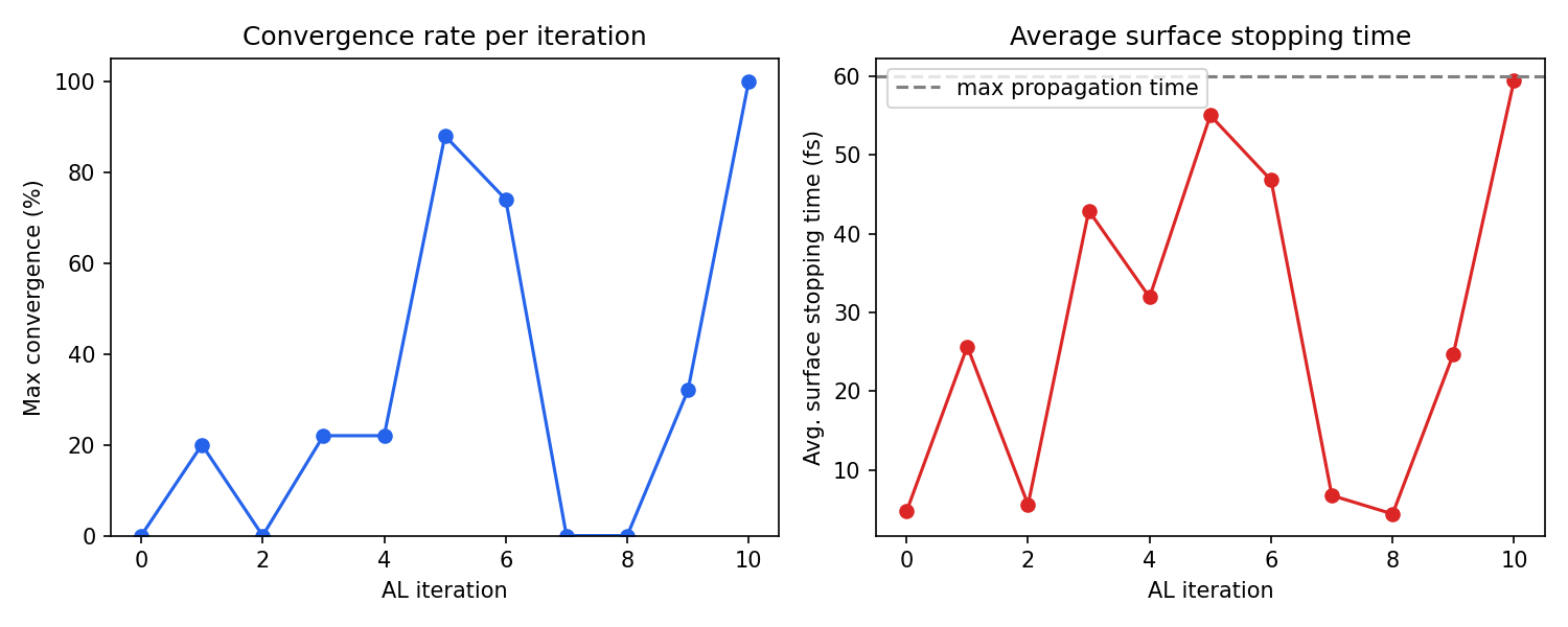
In this fulvene run, the AL loop converged in 10 iterations (iterations 0–10), using a total of 3300 CASSCF-labeled geometries. The convergence was non-monotonic: iterations 5–6 reached about 88% convergence, but iterations 7–8 dropped back to 0% as the newly added data shifted the model’s behavior, requiring further refinement. This is normal and expected. The AL procedure is designed to recover from such regressions by sampling more data in the problematic regions. Final convergence was achieved at iteration 10.
Analyzing the output
The following script parses the AL output log and produces two diagnostic plots:
the maximum convergence rate reached at each iteration
the average surface stopping time, which shows how far trajectories propagate before the model becomes uncertain
"""
Parse an AL-NAMD output log and plot:
    1. Maximum convergence rate (%) per AL iteration
    2. Average surface stopping time (fs) per AL iteration
Usage: python plot_al_convergence.py AL_fulvene.out
"""
import re, sys, matplotlib.pyplot as plt

def parse_al_log(path, ntraj=50, max_time=60.0):
        with open(path) as f:
                text = f.read()
        bounds = [(int(m.group(1)), m.start())
                            for m in re.finditer(r'Active learning iteration (\d+)', text)]
        bounds.append((-1, len(text)))

        iters, max_convs, avg_stops = [], [], []
        for i in range(len(bounds) - 1):
                block = text[bounds[i][1]:bounds[i+1][1]]
                convs = [float(m.group(1))
                                   for m in re.finditer(r'The model is ([\d.]+) % converged', block)]
                # Each convergence check has a stopping-times block listing ONLY uncertain stops.
                # Converged trajectories (reaching max_time) are not listed.
                st_blocks = re.findall(
                        r'The surface stopping times are:\n(.*?)The model is', block, re.DOTALL)
                check_avgs = []
                for j, sb in enumerate(st_blocks):
                        uncertain = [float(x) for x in sb.strip().split('\n') if x.strip()]
                        n_uncertain = len(uncertain)
                        n_converged = ntraj - n_uncertain
                        all_times = uncertain + [max_time] * n_converged
                        check_avgs.append(sum(all_times) / len(all_times))
                iters.append(bounds[i][0])
                max_convs.append(max(convs) if convs else 0)
                avg_stops.append(sum(check_avgs) / len(check_avgs) if check_avgs else 0)
        return iters, max_convs, avg_stops

if __name__ == '__main__':
        path = sys.argv[1] if len(sys.argv) > 1 else 'AL_fulvene.out'
        iters, max_convs, avg_stops = parse_al_log(path)

        fig, (ax1, ax2) = plt.subplots(1, 2, figsize=(10, 4))
        ax1.plot(iters, max_convs, 'o-', color='#2563eb')
        ax1.set_xlabel('AL iteration')
        ax1.set_ylabel('Max convergence (%)')
        ax1.set_ylim(0, 105)
        ax1.set_title('Convergence rate per iteration')

        ax2.plot(iters, avg_stops, 'o-', color='#dc2626')
        ax2.set_xlabel('AL iteration')
        ax2.set_ylabel('Avg. surface stopping time (fs)')
        ax2.set_title('Average surface stopping time')
        ax2.axhline(60, ls='--', color='gray', label='max propagation time')
        ax2.legend()

        plt.tight_layout()
        plt.savefig('al_convergence.png', dpi=150)
        plt.show()
        print('Saved al_convergence.png')
You can run the script above to generate al_convergence.png from the provided AL_fulvene.out log file, see example below:
Additional features
Pre-defined uncertainty thresholds
By default, the uncertainty thresholds are calculated automatically, based on
statistics on the initial data pool. You can provide them yourself within
sampler_kwargs, as a list per-state, or a scalar number for all states.
sampler_kwargs = {
        ...
        'uq_threshold': [0.1, 0.1],  # threshold in Hartree for [S0, S1]
}
This can be useful for tightening the convergence after several iterations.
Providing an initial dataset
Instead of sampling the initial data pool, you can provide it yourself with the following code. Be careful, as this is the dataset that will be used for calculating the thresholds, and it can have a critical impact on accuracy and convergence.
data = ml.data.molecular_database.load('my_existing_data.json', format='json')

ml.al(
        molecule=eqmol,
        initial_dataset=data,
        reference_method=col,
        ...
)
Per-state accuracy breakdown
After upgrading to the latest MLatom version, the training output will include a breakdown of model accuracy (RMSE, correlation coefficient) for each electronic state. This helps diagnose whether the model struggles with a particular state.
Tips and practical advice
GPU memory: Since MLatom version ≥ 3.22 release, the ML models are moved from GPU to CPU during NAMD propagation, preventing VRAM exhaustion from creating multiple copies of model weights across trajectories. If you were previously hitting out-of-memory errors, upgrading should resolve this.
Choosing
new_points: 300 points per iteration is a reasonable default. Fewer points (e.g., 50–100) lead to more iterations but faster individual iterations; more points may be wasteful if many sampled geometries are redundant.Convergence is non-monotonic: Do not be alarmed if convergence drops between iterations. The AL procedure adds data specifically in regions where the model fails, which can temporarily destabilize predictions in other regions. This is by design and the model will recover.
Wall-clock time: For this fulvene example with CASSCF(6,6), the total AL procedure took about 10.5 hours. The dominant cost was training on GPU (iterations with larger datasets take longer). Labeling time with the reference method is influenced by
label_nthreads. However, fulvene is a very simple photophysical system. More complicated, photoreactive molecules can take a lot longer.Using different pre-trained weights: You are not limited to the OMNI-P2x weights. You can provide any compatible
.ptfile. For example, if you have already fine-tuned a model for a similar molecule at the same level of theory, those weights might transfer even better.
References
OMNI-P2x: Mikołaj Martyka, Xin-Yu Tong, Joanna Jankowska, Pavlo Dral. OMNI-P2x: A Universal Neural Network Potential for Excited-State Simulations. ChemRxiv. First posted: 16 April 2025. DOI: https://doi.org/10.26434/chemrxiv-2025-j207x-v2
Active learning for NAMD: Mikołaj Martyka, Lina Zhang, Fuchun Ge, Yi-Fan Hou, Joanna Jankowska*, Mario Barbatti, Pavlo O. Dral. Charting electronic-state manifolds across molecules with multi-state learning and gap-driven dynamics via efficient and robust active learning. npj Comput. Mater. 2025, 11, 132. DOI: https://doi.org/10.1038/s41524-025-01636-z
MLatom surface hopping: Lina Zhang, Sebastian V. Pios, Mikołaj Martyka, Fuchun Ge, Yi-Fan Hou, Yuxinxin Chen, Lipeng Chen, Joanna Jankowska, Mario Barbatti, and Pavlo O. Dral. MLatom Software Ecosystem for Surface Hopping Dynamics in Python with Quantum Mechanical and Machine Learning Methods. J. Chem. Theory Comput. 2024, 20 (12), 5043–5057. DOI: https://doi.org/10.1021/acs.jctc.4c00468